Neural Network with TensorFlow

45 minute read

Published: May 01, 2023

This blog post covers a range of topics related to neural networks and their applications. It begins with an overview of neural network regression and classification using TensorFlow, a popular open-source platform for building and deploying machine learning models. The post then dives into recurrent neural networks, which are specifically designed for processing sequential data, such as time series or natural language. The author highlights the power of RNNs in capturing temporal dependencies and provides a brief tutorial on how to implement an RNN using TensorFlow.

The post is compatible with Google Colaboratory and can be accessed through this link:

Neural Network with TensorFlow

The notebook and examples are developed by Armin Norouzi

Table of Contents:

Neural Network Regression with TensorFlow
Neural Network Classification with TensorFlow
Recurent Neural Network with TensorFlow

Neural Network Regression with TensorFlow

Typical architecture of a regresison neural network

The word typical is on purpose! Because there are many different ways (actually, there’s almost an infinite number of ways) to write neural networks.

But the following is a generic setup for ingesting a collection of numbers, finding patterns in them and then outputing some kind of target number.

Yes, the previous sentence is vague but we’ll see this in action shortly.

Hyperparameter	Typical value
Input layer shape	Same shape as number of features (e.g. 3 for # bedrooms, # bathrooms, # car spaces in housing price prediction)
Hidden layer(s)	Problem specific, minimum = 1, maximum = unlimited
Neurons per hidden layer	Problem specific, generally 10 to 100
Output layer shape	Same shape as desired prediction shape (e.g. 1 for house price)
Hidden activation	Usually ReLU (rectified linear unit)
Output activation	None, ReLU, logistic/tanh
Loss function	MSE (mean square error) or MAE (mean absolute error)/Huber (combination of MAE/MSE) if outliers
Optimizer	SGD (stochastic gradient descent), Adam

Table 1: Typical architecture of a regression network. Source: Adapted from page 293 of Hands-On Machine Learning with Scikit-Learn, Keras & TensorFlow Book by Aurélien Géron

To use TensorFlow, we will import it as the common alias tf (short for TensorFlow).

import tensorflow as tf
print(tf.__version__) # check the version (should be 2.x+)

2.8.2

Regression input shapes and output shapes

One of the most important concepts when working with neural networks are the input and output shapes.

The input shape is the shape of your data that goes into the model.

The output shape is the shape of your data you want to come out of your model.

These will differ depending on the problem you’re working on.

Neural networks accept numbers and output numbers. These numbers are typically represented as tensors (or arrays).

Before, we created data using NumPy arrays, but we could do the same with tensors.

Let’s create a simple data set first and then we can model our NOx model similar to prevous lectures

Simple regression model

Create dataset

import numpy as np
import matplotlib.pyplot as plt

# Make inputs
X = np.arange(-100, 100, 4)


# Make labels for the dataset (y = x + 10)
y = np.arange(-90, 110, 4)

# we used y = x  + 10 to create labels and NN will approximate this function

Split data into training/test set

Training set - the model learns from this data, which is typically 70-80% of the total data available (like the course materials you study during the semester).
Validation set - the model gets tuned on this data, which is typically 10-15% of the total data available (like the practice exam you take before the final exam).
Test set - the model gets evaluated on this data to test what it has learned, it’s typically 10-15% of the

# Check how many samples we have
len(X)

# Split data into train and test sets
X_train = X[:40] # first 40 examples (80% of data)
y_train = y[:40]

X_test = X[40:] # last 10 examples (20% of data)
y_test = y[40:]

len(X_train), len(X_test)

(40, 10)

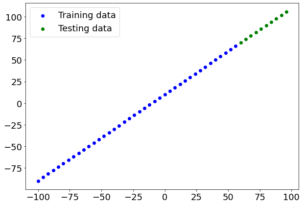
Visualizing the data

plt.figure(figsize=(10, 7))
# Plot training data in blue
plt.scatter(X_train, y_train, c='b', label='Training data')
# Plot test data in green
plt.scatter(X_test, y_test, c='g', label='Testing data')
# Show the legend
plt.legend();

png

Bulding model

Now we know what data we have as well as the input and output shapes, let’s see how we’d build a neural network to model it.

In TensorFlow, there are typically 3 fundamental steps to creating and training a model.

Creating a model - piece together the layers of a neural network yourself (using the Functional or Sequential API) or import a previously built model (known as transfer learning).
Compiling a model - defining how a models performance should be measured (loss/metrics) as well as defining how it should improve (optimizer).
Fitting a model - letting the model try to find patterns in the data (how does X get to y).

Let’s see these in action using the Keras Sequential API to build a model for our regression data. And then we’ll step through each.

Note: If you’re using TensorFlow 2.7.0+, the fit() function no longer upscales input data to go from (batch_size, ) to (batch_size, 1). To fix this, you’ll need to expand the dimension of input data using tf.expand_dims(input_data, axis=-1).
In our case, this means instead of using model.fit(X, y, epochs=5), use model.fit(tf.expand_dims(X, axis=-1), y, epochs=5).

# Set random seed for reproducing purpuse
tf.random.set_seed(42)

# Create a model (same as above)
model = tf.keras.Sequential([
  tf.keras.layers.Dense(1, input_shape=[1]) # define the input_shape to our model
])


# Compile model (same as above)
model.compile(loss=tf.keras.losses.mae, # mae is short for mean absolute error
              optimizer=tf.keras.optimizers.SGD(), # SGD is short for stochastic gradient descent
              metrics=["mae"])

# Summary of model
model.summary()

Model: "sequential_5"
_________________________________________________________________
 Layer (type)                Output Shape              Param #
=================================================================
 dense_9 (Dense)             (None, 1)                 2

=================================================================
Total params: 2
Trainable params: 2
Non-trainable params: 0
_________________________________________________________________

Calling summary() on our model shows us the layers it contains, the output shape and the number of parameters.

Total params - total number of parameters in the model.
Trainable parameters - these are the parameters (patterns) the model can update as it trains.
Non-trainable parameters - these parameters aren’t updated during training (this is typical when you bring in the already learned patterns from other models during transfer learning).

from tensorflow.keras.utils import plot_model

plot_model(model, show_shapes=True)

png

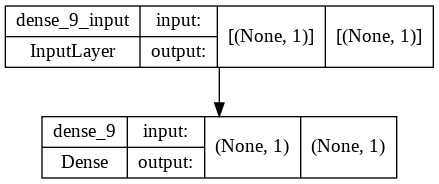
Alongside summary, you can also view a 2D plot of the model using plot_model().

Question: What’s Keras? I thought we were working with TensorFlow but every time we write TensorFlow code, keras comes after tf (e.g. tf.keras.layers.Dense())?

Before TensorFlow 2.0+, Keras was an API designed to be able to build deep learning models with ease. Since TensorFlow 2.0+, its functionality has been tightly integrated within the TensorFlow library.

Question: What’s Dense?

Just your regular densely-connected NN layer. Here is definition if TF documentation (tf.keras.layers.Dense)

tf.keras.layers.Dense(
    units, activation=None, use_bias=True,
    kernel_initializer='glorot_uniform',
    bias_initializer='zeros', kernel_regularizer=None,
    bias_regularizer=None, activity_regularizer=None, kernel_constraint=None,
    bias_constraint=None, **kwargs
)

Let’s fit our model to data

# Fit model
model.fit(tf.expand_dims(X, axis=-1), y, epochs=10)

Epoch 1/10
2/2 [==============================] - 0s 8ms/step - loss: 19.0311 - mae: 19.0311
Epoch 2/10
2/2 [==============================] - 0s 24ms/step - loss: 10.8111 - mae: 10.8111
Epoch 3/10
2/2 [==============================] - 0s 9ms/step - loss: 14.5005 - mae: 14.5005
Epoch 4/10
2/2 [==============================] - 0s 5ms/step - loss: 10.0958 - mae: 10.0958
Epoch 5/10
2/2 [==============================] - 0s 4ms/step - loss: 15.5388 - mae: 15.5388
Epoch 6/10
2/2 [==============================] - 0s 8ms/step - loss: 11.8626 - mae: 11.8626
Epoch 7/10
2/2 [==============================] - 0s 8ms/step - loss: 9.1727 - mae: 9.1727
Epoch 8/10
2/2 [==============================] - 0s 14ms/step - loss: 13.6143 - mae: 13.6143
Epoch 9/10
2/2 [==============================] - 0s 9ms/step - loss: 13.8577 - mae: 13.8577
Epoch 10/10
2/2 [==============================] - 0s 6ms/step - loss: 9.9966 - mae: 9.9966





<keras.callbacks.History at 0x7f79b029d050>

Not that much improvement!

Evaluating model

A typical workflow you’ll go through when building neural networks is:

Build a model -> evaluate it -> build (tweak) a model -> evaulate it -> build (tweak) a model -> evaluate it...

The tweaking comes from maybe not building a model from scratch but adjusting an existing one.

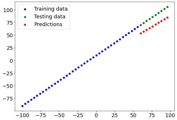
# Make predictions
y_preds = model.predict(X_test)

Function for plotting

def plot_predictions(train_data=X_train,
                     train_labels=y_train,
                     test_data=X_test,
                     test_labels=y_test,
                     predictions=y_preds):
  """
  Plots training data, test data and compares predictions.
  """
  plt.figure(figsize=(10, 7))
  # Plot training data in blue
  plt.scatter(train_data, train_labels, c="b", label="Training data")
  # Plot test data in green
  plt.scatter(test_data, test_labels, c="g", label="Testing data")
  # Plot the predictions in red (predictions were made on the test data)
  plt.scatter(test_data, predictions, c="r", label="Predictions")
  # Show the legend
  plt.legend();

plot_predictions(train_data=X_train,
                 train_labels=y_train,
                 test_data=X_test,
                 test_labels=y_test,
                 predictions=y_preds)

png

Very poor model! We can now add neurons and layers to make a more sophisticated model!

Alongisde visualizations, evaulation metrics are your alternative best option for evaluating your model.

Depending on the problem you’re working on, different models have different evaluation metrics.

Two of the main metrics used for regression problems are:

Mean absolute error (MAE) - the mean difference between each of the predictions.
Mean squared error (MSE) - the squared mean difference between of the predictions (use if larger errors are more detrimental than smaller errors).

The lower each of these values, the better.

You can also use model.evaluate() which will return the loss of the model as well as any metrics setup during the compile step.

# Evaluate the model on the test set
model.evaluate(X_test, y_test)

1/1 [==============================] - 0s 127ms/step - loss: 11.4078 - mae: 11.4078

[11.407841682434082, 11.407841682434082]

In our case, since we used MAE for the loss function as well as MAE for the metrics, model.evaulate() returns them both.

TensorFlow also has built in functions for MSE and MAE.

For many evaluation functions, the premise is the same: compare predictions to the ground truth labels.

We can create function to calculate MAE and MSE:

def mae(y_test, y_pred):
  """
  Calculuates mean absolute error between y_test and y_preds.
  """
  return tf.metrics.mean_absolute_error(y_test,
                                        y_pred)

def mse(y_test, y_pred):
  """
  Calculates mean squared error between y_test and y_preds.
  """
  return tf.metrics.mean_squared_error(y_test,
                                       y_pred)

mae(y_test, y_preds), mse(y_test, y_preds)

(<tf.Tensor: shape=(10,), dtype=float32, numpy=
 array([29.051418, 25.130623, 21.209831, 17.431225, 14.420944, 12.178976,
        10.70533 , 10.      , 10.062988, 10.894293], dtype=float32)>,
 <tf.Tensor: shape=(10,), dtype=float32, numpy=
 array([975.98486, 763.54816, 581.85693, 430.91064, 310.70984, 221.25415,
        162.54385, 134.57878, 137.35895, 170.88437], dtype=float32)>)

That’s strange, MAE should be a single output.

Instead, we get 10 values!

This is because our y_test and y_preds tensors are different shapes.

# Check the tensor shapes
y_test.shape, y_preds.shape

((10,), (10, 1))

We can fix it using squeeze(), it’ll remove the the 1 dimension from our y_preds tensor, making it the same shape as y_test.

# Check the tensor shapes
y_test.shape, y_preds.squeeze().shape

((10,), (10,))

mae(y_test, y_preds.squeeze()), mse(y_test, y_preds.squeeze())

(<tf.Tensor: shape=(), dtype=float32, numpy=11.407842>,
 <tf.Tensor: shape=(), dtype=float32, numpy=130.19061>)

MAE is 17.27 and MSE is 300.03 for test dataset.

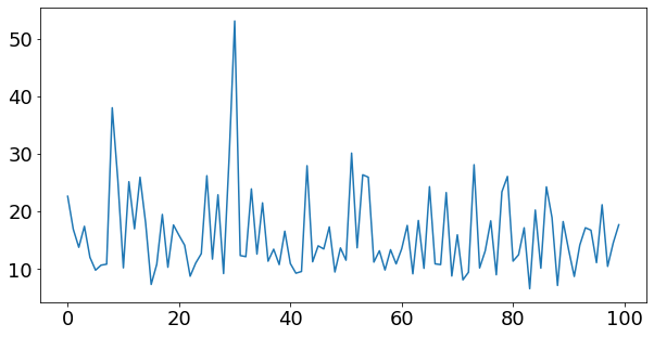
Plotting loss vs epochs

Before trying to improve model, let’s learn how to plot loss vs epochs
To do this, we need to assign model.fit to a variable such as history

history = model.fit(tf.expand_dims(X, axis=-1), y, epochs=100, verbose = 0) # verbose = 0 means do not show iterations

Evaluation of history:

history.history.keys()

dict_keys(['loss', 'mae'])

So we can plot both loss and metrics we defined in compile using history

plt.figure(figsize=(10,5))
plt.plot(history.history['loss'])

[<matplotlib.lines.Line2D at 0x7f79aca8b8d0>]

png

Running experiments to improve a model

After seeing the evaluation metrics and the predictions your model makes, it’s likely you’ll want to improve it.

Again, there are many different ways you can do this, but 3 of the main ones are:

Get more data - get more examples for your model to train on (more opportunities to learn patterns).
Make your model larger (use a more complex model) - this might come in the form of more layers or more hidden units in each layer.
Train for longer - give your model more of a chance to find the patterns in the data.

Since we created our dataset, we could easily make more data but this isn’t always the case when you’re working with real-world datasets.

So let’s take a look at how we can improve our model using 2 and 3.

To do so, we’ll build 3 models and compare their results:

model_1 - same as original model, 1 layer, trained for 100 epochs.
model_2 - 2 layers, trained for 100 epochs.
model_3 - 2 layers, trained for 500 epochs.

Build model_1

# Set random seed
tf.random.set_seed(42)

# Replicate original model
model_1 = tf.keras.Sequential([
  tf.keras.layers.Dense(1)
])

# Compile the model
model_1.compile(loss=tf.keras.losses.mae,
                optimizer=tf.keras.optimizers.SGD(),
                metrics=['mae'])

# Fit the model
history_1 = model_1.fit(tf.expand_dims(X_train, axis=-1), y_train, epochs=100, verbose = 0)


plt.figure(figsize=(10,5))
plt.plot(history_1.history['loss'])

[<matplotlib.lines.Line2D at 0x7f79b11af410>]

png

# Make and plot predictions for model_1
y_preds_1 = model_1.predict(X_test)
plot_predictions(predictions=y_preds_1)

png

# Calculate model_1 metrics
mae_1 = mae(y_test, y_preds_1.squeeze()).numpy()
mse_1 = mse(y_test, y_preds_1.squeeze()).numpy()
mae_1, mse_1

(18.745327, 353.57336)

Build model_2

This time we’ll add an extra dense layer (so now our model will have 2 layers) whilst keeping everything else the same.

# Set random seed
tf.random.set_seed(42)

# Replicate original model
model_2 = tf.keras.Sequential([
  tf.keras.layers.Dense(1),
  tf.keras.layers.Dense(1) # add a second layer
])

# Compile the model
model_2.compile(loss=tf.keras.losses.mae,
                optimizer=tf.keras.optimizers.SGD(),
                metrics=['mae'])

# Fit the model
history_2 = model_2.fit(tf.expand_dims(X_train, axis=-1), y_train, epochs=100, verbose = 0)


plt.figure(figsize=(10,5))
plt.plot(history_2.history['loss'])

[<matplotlib.lines.Line2D at 0x7f79b0d20b10>]

png

# Make and plot predictions for model_2
y_preds_2 = model_2.predict(X_test)
plot_predictions(predictions=y_preds_2)

png

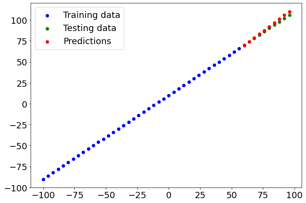
# Calculate model_2 metrics
mae_2 = mae(y_test, y_preds_2.squeeze()).numpy()
mse_2 = mse(y_test, y_preds_2.squeeze()).numpy()
mae_2, mse_2

(1.9098114, 5.459232)

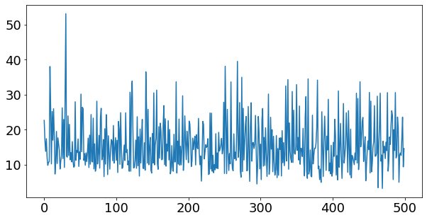
Build model_3

For our 3rd model, we’ll keep everything the same as model_2 except this time we’ll train for longer (500 epochs instead of 100).

This will give our model more of a chance to learn the patterns in the data.

# Set random seed
tf.random.set_seed(42)

# Replicate original model
model_3 = tf.keras.Sequential([
  tf.keras.layers.Dense(1),
  tf.keras.layers.Dense(1) # add a second layer
])

# Compile the model
model_3.compile(loss=tf.keras.losses.mae,
                optimizer=tf.keras.optimizers.SGD(),
                metrics=['mae'])

# Fit the model
history_3 = model_3.fit(tf.expand_dims(X_train, axis=-1), y_train, epochs=500, verbose = 0)


plt.figure(figsize=(10,5))
plt.plot(history_3.history['loss'])

[<matplotlib.lines.Line2D at 0x7f79b0bfccd0>]

png

# Make and plot predictions for model_3
y_preds_3 = model_3.predict(X_test)
plot_predictions(predictions=y_preds_3)

png

# Calculate model_3 metrics
mae_3 = mae(y_test, y_preds_3.squeeze()).numpy()
mse_3 = mse(y_test, y_preds_3.squeeze()).numpy()
mae_3, mse_3

(68.68786, 4804.4717)

Comparing results

Now we’ve got results for 3 similar but slightly different results, let’s compare them.

model_results = [["model_1", mae_1, mse_1],
                 ["model_2", mae_2, mse_2],
                 ["model_3", mae_3, mae_3]]

import pandas as pd
all_results = pd.DataFrame(model_results, columns=["model", "mae", "mse"])
all_results

	model	mae	mse
0	model_1	18.745327	353.573364
1	model_2	1.909811	5.459232
2	model_3	68.687859	68.687859

From our experiments, it looks like model_2 performed the best.

And now, you might be thinking, “wow, comparing models is tedious…” and it definitely can be, we’ve only compared 3 models here.

But this is part of what machine learning modelling is about, trying many different combinations of models and seeing which performs best.

Each model you build is a small experiment.

Saving a model

Once you’ve trained a model and found one which performs to your liking, you’ll probably want to save it for use elsewhere (like a web application or mobile device).

You can save a TensorFlow/Keras model using model.save().

There are two ways to save a model in TensorFlow:

The SavedModel format (default).
The HDF5 format.

The main difference between the two is the SavedModel is automatically able to save custom objects (such as special layers) without additional modifications when loading the model back in.

Which one should you use?

It depends on your situation but the SavedModel format will suffice most of the time.

Both methods use the same method call.

# Save a model using the SavedModel format
model_2.save('best_model_SavedModel_format')

INFO:tensorflow:Assets written to: best_model_SavedModel_format/assets

# Check it out - outputs a protobuf binary file (.pb) as well as other files
!ls best_model_SavedModel_format

assets	keras_metadata.pb  saved_model.pb  variables

Now let’s save the model in the HDF5 format, we’ll use the same method but with a different filename.

# Save a model using the HDF5 format
model_2.save("best_model_HDF5_format.h5") # note the addition of '.h5' on the end

# Check it out
!ls best_model_HDF5_format.h5

best_model_HDF5_format.h5

Loading a model

We can load a saved model using the load_model() method.

Loading a model for the different formats (SavedModel and HDF5) is the same (as long as the pathnames to the particuluar formats are correct).

# Load a model from the SavedModel format
loaded_saved_model = tf.keras.models.load_model("best_model_SavedModel_format")
loaded_saved_model.summary()

Model: "sequential_7"
_________________________________________________________________
 Layer (type)                Output Shape              Param #
=================================================================
 dense_11 (Dense)            (None, 1)                 2

 dense_12 (Dense)            (None, 1)                 2

=================================================================
Total params: 4
Trainable params: 4
Non-trainable params: 0
_________________________________________________________________

Now let’s test it out:

# Compare model_2 with the SavedModel version (should return True)
model_2_preds = model_2.predict(X_test)
saved_model_preds = loaded_saved_model.predict(X_test)

mae(y_test, saved_model_preds.squeeze()).numpy() == mae(y_test, model_2_preds.squeeze()).numpy()

True

Loading in from the HDF5 is much the same.

# Load a model from the HDF5 format
loaded_h5_model = tf.keras.models.load_model("best_model_HDF5_format.h5")
loaded_h5_model.summary()

Model: "sequential_7"
_________________________________________________________________
 Layer (type)                Output Shape              Param #
=================================================================
 dense_11 (Dense)            (None, 1)                 2

 dense_12 (Dense)            (None, 1)                 2

=================================================================
Total params: 4
Trainable params: 4
Non-trainable params: 0
_________________________________________________________________

# Compare model_2 with the loaded HDF5 version (should return True)
h5_model_preds = loaded_h5_model.predict(X_test)

mae(y_test, h5_model_preds.squeeze()).numpy() == mae(y_test, model_2_preds.squeeze()).numpy()

True

Downloading a model (from Google Colab)

Say you wanted to get your model from Google Colab to your local machine, you can do one of the following things:

Right click on the file in the files pane and click ‘download’.
Use the code below.

# Download the model (or any file) from Google Colab
from google.colab import files
files.download("best_model_HDF5_format.h5")

<IPython.core.display.Javascript object>

<IPython.core.display.Javascript object>

Diesel NOx model prediction

Importing data

data = pd.read_csv('https://raw.githubusercontent.com/arminnorouzi/ML-developed_course/main/Data/Engine_NOx_classification.csv')
data.head()

	Load [ft.lb]	Engine speed [rpm]	mf [mg/stroke]	Pr [PSI]	NOx [ppm]
0	50	2502.400000	31.222326	15285.16744	103.899724
1	50	2248.666667	30.116667	15155.13333	112.610181
2	75	2502.000000	38.300000	15356.00000	114.789893
3	100	2504.000000	42.900000	15296.00000	125.411970
4	75	2262.000000	34.100000	15254.00000	126.524679

cdf = data[['Load [ft.lb]','Engine speed [rpm]','mf [mg/stroke]','Pr [PSI]', 'NOx [ppm]']]

msk = np.random.rand(len(data)) < 0.8
train = cdf[msk]
test = cdf[~msk]

font = {'family' : 'normal',
        'weight' : 'normal',
        'size'   : 18}

plt.rc('font', **font)

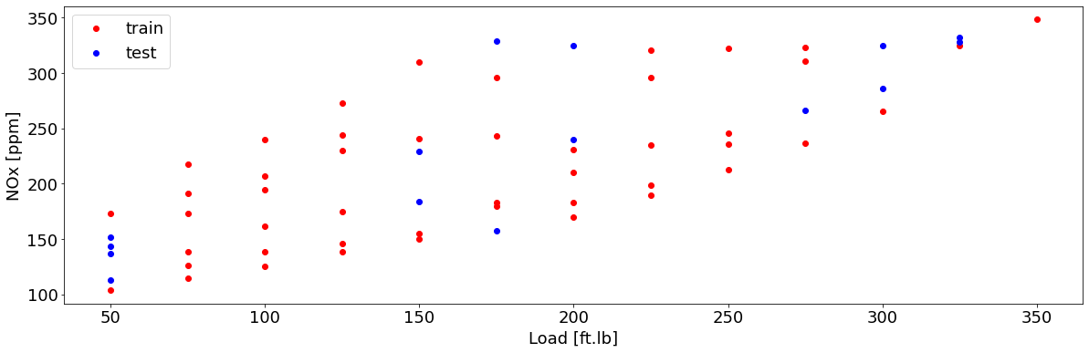
plt.figure(1, figsize=(20, 6))
plt.plot(train['Load [ft.lb]'], train['NOx [ppm]'], 'or', label = 'train')
plt.plot(test['Load [ft.lb]'], test['NOx [ppm]'], 'ob', label = 'test')
plt.xlabel('Load [ft.lb]', fontsize=18)
plt.ylabel('NOx [ppm]', fontsize=18)
plt.legend(fontsize=18)

<matplotlib.legend.Legend at 0x7f79b08c2dd0>

png

Train/test set

from sklearn import preprocessing

x_train = np.asanyarray(train[['Load [ft.lb]','Engine speed [rpm]','mf [mg/stroke]','Pr [PSI]']])

x_test = np.asanyarray(test[['Load [ft.lb]','Engine speed [rpm]','mf [mg/stroke]','Pr [PSI]']])

# train_x = np.asanyarray(train[['Load [ft.lb]','Engine speed [rpm]']])
y_train = np.asanyarray(train[['NOx [ppm]']])

# test_x = np.asanyarray(test[['Load [ft.lb]','Engine speed [rpm]']])
y_test = np.asanyarray(test[['NOx [ppm]']])


min_max_scaler = preprocessing.MinMaxScaler()
X_train_minmax = min_max_scaler.fit_transform(x_train)
X_test_minmax = min_max_scaler.transform(x_test)

Define model: Here similar model with one hidden layer with 15 neuron will be used as a first try

# 1. Create model using the sequential API

NOx_model = tf.keras.Sequential([
                      tf.keras.layers.Dense(1, input_shape = [4], name ="Input_layer"),
                      tf.keras.layers.Dense(15, activation="relu", name ="Hidden_layer_1"),
                      tf.keras.layers.Dense(1, name = "Output_layer")
                      ], name = "My_NN_model")

# 2. Compile model

NOx_model.compile(loss = tf.keras.losses.mae,
              optimizer = tf.keras.optimizers.Adam(learning_rate = 0.01), #here Adam optimizer is used
              metrics = ["mae"])

NOx_model.summary()

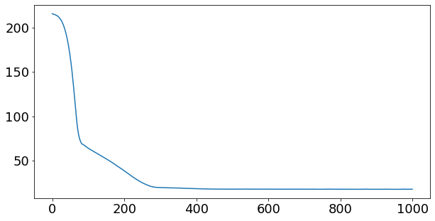
history = NOx_model.fit(X_train_minmax,y_train, epochs = 1000,verbose = 0)

plt.figure(figsize=(10,5))
plt.plot(history.history['loss'])

Model: "My_NN_model"
_________________________________________________________________
 Layer (type)                Output Shape              Param #
=================================================================
 Input_layer (Dense)         (None, 1)                 5

 Hidden_layer_1 (Dense)      (None, 15)                30

 Output_layer (Dense)        (None, 1)                 16

=================================================================
Total params: 51
Trainable params: 51
Non-trainable params: 0
_________________________________________________________________





[<matplotlib.lines.Line2D at 0x7f79b095acd0>]

png

train_y_hat = NOx_model.predict(X_train_minmax)
test_y_hat = NOx_model.predict(X_test_minmax)

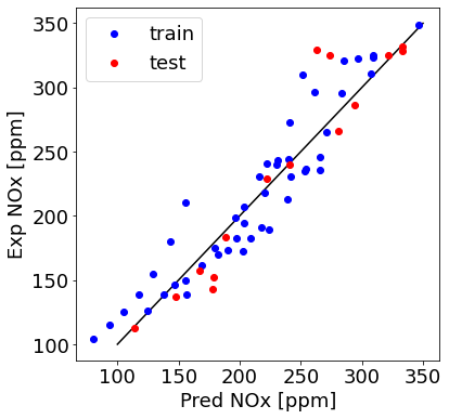
plt.figure(1, figsize=(6, 6))
plt.plot([100,350], [100, 350],  '-k')
plt.plot(train_y_hat, train['NOx [ppm]'], 'ob', label = 'train')
plt.plot(test_y_hat, test['NOx [ppm]'], 'or', label = 'test')
plt.ylabel("Exp NOx [ppm]", fontsize=18)
plt.xlabel("Pred NOx [ppm]", fontsize=18)
plt.legend(fontsize=18)

<matplotlib.legend.Legend at 0x7f79b073dad0>

png

Improving the mode

adding more layer

# 1. Create model using the sequential API

NOx_model = tf.keras.Sequential([
                      tf.keras.layers.Dense(1, input_shape = [4], name ="Input_layer"),
                      tf.keras.layers.Dense(15, activation="relu", name ="Hidden_layer_1"),
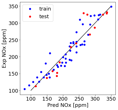
                      tf.keras.layers.Dense(15, activation="relu", name ="Hidden_layer_2"),
                      tf.keras.layers.Dense(1, name = "Output_layer")
                      ], name = "My_NN_model")

# 2. Compile model

NOx_model.compile(loss = tf.keras.losses.mae,
              optimizer = tf.keras.optimizers.Adam(learning_rate = 0.01), #here Adam optimizer is used
              metrics = ["mae"])

NOx_model.summary()

history = NOx_model.fit(X_train_minmax,y_train, epochs = 1000,verbose = 0)

plt.figure(figsize=(10,5))
plt.plot(history.history['loss'])

Model: "My_NN_model"
_________________________________________________________________
 Layer (type)                Output Shape              Param #
=================================================================
 Input_layer (Dense)         (None, 1)                 5

 Hidden_layer_1 (Dense)      (None, 15)                30

 Hidden_layer_2 (Dense)      (None, 15)                240

 Output_layer (Dense)        (None, 1)                 16

=================================================================
Total params: 291
Trainable params: 291
Non-trainable params: 0
_________________________________________________________________





[<matplotlib.lines.Line2D at 0x7f79b06865d0>]

png

train_y_hat = NOx_model.predict(X_train_minmax)
test_y_hat = NOx_model.predict(X_test_minmax)


plt.figure(1, figsize=(6, 6))
plt.plot([100,350], [100, 350],  '-k')
plt.plot(train_y_hat, train['NOx [ppm]'], 'ob', label = 'train')
plt.plot(test_y_hat, test['NOx [ppm]'], 'or', label = 'test')
plt.ylabel("Exp NOx [ppm]", fontsize=18)
plt.xlabel("Pred NOx [ppm]", fontsize=18)
plt.legend(fontsize=18)

<matplotlib.legend.Legend at 0x7f79af8149d0>

png

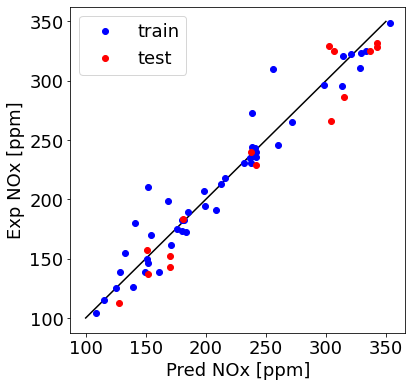
This is a good model! Can we add regularization in tensorflow
Regularizers allow you to apply penalties on layer parameters or layer activity during optimization. These penalties are summed into the loss function that the network optimizes.

Regularization penalties are applied on a per-layer basis. The exact API will depend on the layer, but many layers (e.g. Dense, Conv1D, Conv2D and Conv3D) have a unified API.

These layers expose 3 keyword arguments:

kernel_regularizer: Regularizer to apply a penalty on the layer’s kernel
bias_regularizer: Regularizer to apply a penalty on the layer’s bias
activity_regularizer: Regularizer to apply a penalty on the layer’s output

All layers (including custom layers) expose activity_regularizer as a settable property, whether or not it is in the constructor arguments.

The value returned by the activity_regularizer is divided by the input batch size so that the relative weighting between the weight regularizers and the activity regularizers does not change with the batch size.

You can access a layer’s regularization penalties by calling layer.losses after calling the layer on inputs.

Available penalties

tf.keras.regularizers.L1(0.3)  # L1 Regularization Penalty
tf.keras.regularizers.L2(0.1)  # L2 Regularization Penalty
tf.keras.regularizers.L1L2(l1=0.01, l2=0.01)  # L1 + L2 penalties

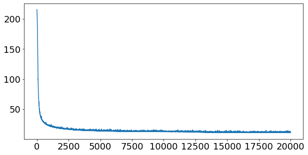
As we add regularization, we can increase layer size with less chance of overfitting:

# 1. Create model using the sequential API

NOx_model = tf.keras.Sequential([
                      tf.keras.layers.Dense(1, input_shape = [4], name ="Input_layer"),
                      tf.keras.layers.Dense(45, activation="relu", name ="Hidden_layer_1", activity_regularizer=tf.keras.regularizers.L2(0.1)), # L2 regularization is added
                      tf.keras.layers.Dense(15, activation="relu", name ="Hidden_layer_2", activity_regularizer=tf.keras.regularizers.L2(0.1)),
                      tf.keras.layers.Dense(1, name = "Output_layer")
                      ], name = "My_NN_model")

# 2. Compile model

NOx_model.compile(loss = tf.keras.losses.mae,
              optimizer = tf.keras.optimizers.Adam(learning_rate = 0.01), #here Adam optimizer is used
              metrics = ["mae"])

NOx_model.summary()

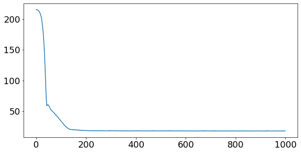
history = NOx_model.fit(X_train_minmax,y_train, epochs = 20000,verbose = 0)

plt.figure(figsize=(10,5))
plt.plot(history.history['loss'])

Model: "My_NN_model"
_________________________________________________________________
 Layer (type)                Output Shape              Param #
=================================================================
 Input_layer (Dense)         (None, 1)                 5

 Hidden_layer_1 (Dense)      (None, 45)                90

 Hidden_layer_2 (Dense)      (None, 15)                690

 Output_layer (Dense)        (None, 1)                 16

=================================================================
Total params: 801
Trainable params: 801
Non-trainable params: 0
_________________________________________________________________





[<matplotlib.lines.Line2D at 0x7f79af43d750>]

png

train_y_hat = NOx_model.predict(X_train_minmax)
test_y_hat = NOx_model.predict(X_test_minmax)


plt.figure(1, figsize=(6, 6))
plt.plot([100,350], [100, 350],  '-k')
plt.plot(train_y_hat, train['NOx [ppm]'], 'ob', label = 'train')
plt.plot(test_y_hat, test['NOx [ppm]'], 'or', label = 'test')
plt.ylabel("Exp NOx [ppm]", fontsize=18)
plt.xlabel("Pred NOx [ppm]", fontsize=18)
plt.legend(fontsize=18)

<matplotlib.legend.Legend at 0x7f79af381210>

png

Neural Network Classification with TensorFlow

Okay, we’ve seen how to deal with a regression problem in TensorFlow, let’s look at how we can approach a classification problem.

A classification problem involves predicting whether something is one thing or another.

For example, you might want to:

Predict whether or not someone has heart disease based on their health parameters. This is called binary classification since there are only two options.
Decide whether a photo of is of food, a person or a dog. This is called multi-class classification since there are more than two options.
Predict what categories should be assigned to a Wikipedia article. This is called multi-label classification since a single article could have more than one category assigned.

In this notebook, we’re going to work through a number of different classification problems with TensorFlow. In other words, taking a set of inputs and predicting what class those set of inputs belong to.

Typical architecture of a classification neural network

The word typical is on purpose. Because the architecture of a classification neural network can widely vary depending on the problem you’re working on.

However, there are some fundamentals all deep neural networks contain:

An input layer.
Some hidden layers.
An output layer.

Much of the rest is up to the data analyst creating the model.

The following are some standard values you’ll often use in your classification neural networks.

Hyperparameter	Binary Classification	Multiclass classification
Input layer shape	Same as number of features (e.g. 5 for age, sex, height, weight, smoking status in heart disease prediction)	Same as binary classification
Hidden layer(s)	Problem specific, minimum = 1, maximum = unlimited	Same as binary classification
Neurons per hidden layer	Problem specific, generally 10 to 100	Same as binary classification
Output layer shape	1 (one class or the other)	1 per class (e.g. 3 for food, person or dog photo)
Hidden activation	Usually ReLU (rectified linear unit)	Same as binary classification
Output activation	Sigmoid	Softmax
Loss function	Cross entropy (`tf.keras.losses.BinaryCrossentropy` in TensorFlow)	Cross entropy (`tf.keras.losses.CategoricalCrossentropy` in TensorFlow)
Optimizer	SGD (stochastic gradient descent), Adam	Same as binary classification

Table 1: Typical architecture of a classification network. Source: Adapted from page 295 of Hands-On Machine Learning with Scikit-Learn, Keras & TensorFlow Book by Aurélien Géron

Creating data to view and fit

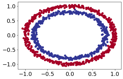
We could start by importing a classification dataset but let’s practice making some of our own classification data.

Since classification is predicting whether something is one thing or another, let’s make some data to reflect that.

To do so, we’ll use Scikit-Learn’s make_circles() function.

from sklearn.datasets import make_circles

# Make 1000 examples
n_samples = 1000

# Create circles
X, y = make_circles(n_samples,
                    noise=0.03,
                    random_state=42)

# Make dataframe of features and labels
import pandas as pd
circles = pd.DataFrame({"X0":X[:, 0], "X1":X[:, 1], "label":y})
circles.head()

	X0	X1	label
0	0.754246	0.231481	1
1	-0.756159	0.153259	1
2	-0.815392	0.173282	1
3	-0.393731	0.692883	1
4	0.442208	-0.896723	0

What kind of labels are we dealing with?

# Check out the different labels
circles.label.value_counts()

1    500
0    500
Name: label, dtype: int64

Alright, looks like we’re dealing with a binary classification problem. It’s binary because there are only two labels (0 or 1).

If there were more label options (e.g. 0, 1, 2, 3 or 4), it would be called multiclass classification.

Let’s take our visualization a step further and plot our data.

# Visualize with a plot
import matplotlib.pyplot as plt
plt.scatter(X[:, 0], X[:, 1], c=y, cmap=plt.cm.RdYlBu);

png

Input and output shapes

One of the most common issues you’ll run into when building neural networks is shape mismatches.

More specifically, the shape of the input data and the shape of the output data.

In our case, we want to input X and get our model to predict y.

So let’s check out the shapes of X and y.

# Check the shapes of our features and labels
X.shape, y.shape

((1000, 2), (1000,))

# Check how many samples we have
len(X), len(y)

(1000, 1000)

To visualize our model’s predictions we’re going to create a function plot_decision_boundary() which:

Takes in a trained model, features (X) and labels (y).
Creates a meshgrid of the different X values.
Makes predictions across the meshgrid.
Plots the predictions as well as a line between the different zones (where each unique class falls).

import numpy as np

def plot_decision_boundary(model, X, y):
  """
  Plots the decision boundary created by a model predicting on X.
  This function has been adapted from two phenomenal resources:
   1. CS231n - https://cs231n.github.io/neural-networks-case-study/
   2. Made with ML basics - https://github.com/GokuMohandas/MadeWithML/blob/main/notebooks/08_Neural_Networks.ipynb
  """
  # Define the axis boundaries of the plot and create a meshgrid
  x_min, x_max = X[:, 0].min() - 0.1, X[:, 0].max() + 0.1
  y_min, y_max = X[:, 1].min() - 0.1, X[:, 1].max() + 0.1
  xx, yy = np.meshgrid(np.linspace(x_min, x_max, 100),
                       np.linspace(y_min, y_max, 100))

  # Create X values (we're going to predict on all of these)
  x_in = np.c_[xx.ravel(), yy.ravel()] # stack 2D arrays together: https://numpy.org/devdocs/reference/generated/numpy.c_.html

  # Make predictions using the trained model
  y_pred = model.predict(x_in)

  # Check for multi-class
  if len(y_pred[0]) > 1:
    print("doing multiclass classification...")
    # We have to reshape our predictions to get them ready for plotting
    y_pred = np.argmax(y_pred, axis=1).reshape(xx.shape)
  else:
    print("doing binary classifcation...")
    y_pred = np.round(y_pred).reshape(xx.shape)

  # Plot decision boundary
  plt.contourf(xx, yy, y_pred, cmap=plt.cm.RdYlBu, alpha=0.7)
  plt.scatter(X[:, 0], X[:, 1], c=y, s=40, cmap=plt.cm.RdYlBu)
  plt.xlim(xx.min(), xx.max())
  plt.ylim(yy.min(), yy.max())

Steps in modelling

Now we know what data we have as well as the input and output shapes, let’s see how we’d build a neural network to model it.

In TensorFlow, there are typically 3 fundamental steps to creating and training a model.

Creating a model - piece together the layers of a neural network yourself (using the functional or sequential API) or import a previously built model (known as transfer learning).
Compiling a model - defining how a model’s performance should be measured (loss/metrics) as well as defining how it should improve (optimizer).
Fitting a model - letting the model try to find patterns in the data (how does X get to y).

Let’s see these in action using the Sequential API to build a model for our regression data. And then we’ll step through each.

# Let's try with linear activation function

# Set random seed
tf.random.set_seed(42)

# Create a model
model_1 = tf.keras.Sequential([
  tf.keras.layers.Dense(4, activation="relu", name ="Input_Layer"), # hidden layer 1, 4 neurons, ReLU activation
  tf.keras.layers.Dense(4, activation="relu", name ="Hidden_layer_1"), # hidden layer 2, 4 neurons, ReLU activation
  tf.keras.layers.Dense(1, name ="Output_layer")], name = "My_NN_classification_model")

# Compile the model
model_1.compile(loss=tf.keras.losses.binary_crossentropy,
                optimizer=tf.keras.optimizers.Adam(learning_rate=0.001), # Adam's default learning rate is 0.001
                metrics=['accuracy'])



# Fit the model
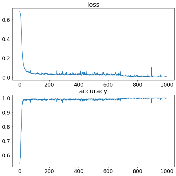
history = model_1.fit(X, y, epochs=100, verbose = 0)
model_1.summary()


plt.figure(figsize=(10,10))
plt.subplot(2, 1, 1)
plt.plot(history.history['loss'])
plt.title("loss")
plt.subplot(2, 1, 2)
plt.plot(history.history['accuracy'])
plt.title("accuracy")
plt.show()

model_1.evaluate(X,y)

Model: "My_NN_classification_model"
_________________________________________________________________
 Layer (type)                Output Shape              Param #
=================================================================
 Input_Layer (Dense)         (None, 4)                 12

 Hidden_layer_1 (Dense)      (None, 4)                 20

 Output_layer (Dense)        (None, 1)                 5

=================================================================
Total params: 37
Trainable params: 37
Non-trainable params: 0
_________________________________________________________________

png

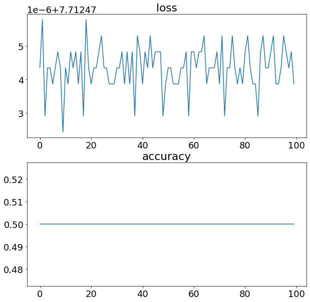
32/32 [==============================] - 0s 1ms/step - loss: 7.7125 - accuracy: 0.5000

[7.712474346160889, 0.5]

# View the predictions of the model
plot_decision_boundary(model_1, X, y)

doing binary classifcation...

png

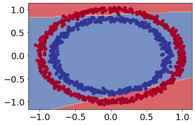
Looks like our model is trying to draw a straight line through the data.

What’s wrong with doing this?

The main issue is our data isn’t separable by a straight line. So we need to add activation function to add nonlinearities in our model

# Let's try with sigmoid activation function

# Set random seed
tf.random.set_seed(42)

# Create a model
model_2 = tf.keras.Sequential([
  tf.keras.layers.Dense(4, activation="relu", name ="Input_Layer"), # hidden layer 1, ReLU activation
  tf.keras.layers.Dense(4, activation="relu", name ="Hidden_layer_1"), # hidden layer 2, ReLU activation
  tf.keras.layers.Dense(1, activation="sigmoid", name ="Output_Layer") # ouput layer, sigmoid activation
], name = "My_NN_classification_model")

# Compile the model
model_2.compile(loss=tf.keras.losses.binary_crossentropy,
                optimizer=tf.keras.optimizers.Adam(learning_rate=0.01),
                metrics=['accuracy'])



# Fit the model
history = model_2.fit(X, y, epochs=1000, verbose=0)

model_2.summary()


plt.figure(figsize=(10,10))
plt.subplot(2, 1, 1)
plt.plot(history.history['loss'])
plt.title("loss")
plt.subplot(2, 1, 2)
plt.plot(history.history['accuracy'])
plt.title("accuracy")
plt.show()

model_2.evaluate(X,y)

Model: "My_NN_classification_model"
_________________________________________________________________
 Layer (type)                Output Shape              Param #
=================================================================
 Input_Layer (Dense)         (None, 4)                 12

 Hidden_layer_1 (Dense)      (None, 4)                 20

 Output_Layer (Dense)        (None, 1)                 5

=================================================================
Total params: 37
Trainable params: 37
Non-trainable params: 0
_________________________________________________________________

png

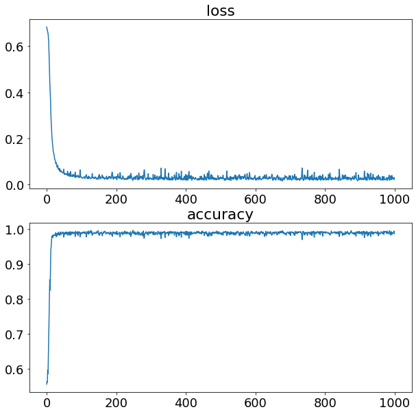
32/32 [==============================] - 0s 3ms/step - loss: 0.0244 - accuracy: 0.9890

[0.024428997188806534, 0.9890000224113464]

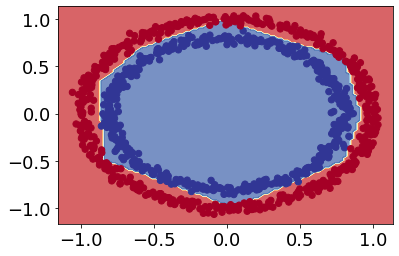
# View the predictions of the model
plot_decision_boundary(model_2, X, y)

doing binary classifcation...

png

Evaluating and improving our classification model

# Split data into train and test sets
X_train, y_train = X[:800], y[:800] # 80% of the data for the training set
X_test, y_test = X[800:], y[800:] # 20% of the data for the test set

# Check the shapes of the data
X_train.shape, X_test.shape # 800 examples in the training set, 200 examples in the test set

((800, 2), (200, 2))

# Let's try with sigmoid activation function

# Set random seed
tf.random.set_seed(42)

# Create a model
model_3 = tf.keras.Sequential([
  tf.keras.layers.Dense(4, activation="relu", name ="Input_Layer"), # hidden layer 1, ReLU activation
  tf.keras.layers.Dense(4, activation="relu", name ="Hidden_layer_1"), # hidden layer 2, ReLU activation
  tf.keras.layers.Dense(1, activation="sigmoid", name ="Output_Layer") # ouput layer, sigmoid activation
], name = "My_NN_classification_model")

# Compile the model
model_3.compile(loss=tf.keras.losses.binary_crossentropy,
                optimizer=tf.keras.optimizers.Adam(learning_rate=0.01),
                metrics=['accuracy'])



# Fit the model
history = model_3.fit(X_train, y_train, epochs=1000, verbose=0)

model_3.summary()


plt.figure(figsize=(10,10))
plt.subplot(2, 1, 1)
plt.plot(history.history['loss'])
plt.title("loss")
plt.subplot(2, 1, 2)
plt.plot(history.history['accuracy'])
plt.title("accuracy")
plt.show()

Model: "My_NN_classification_model"
_________________________________________________________________
 Layer (type)                Output Shape              Param #
=================================================================
 Input_Layer (Dense)         (32, 4)                   12

 Hidden_layer_1 (Dense)      (32, 4)                   20

 Output_Layer (Dense)        (32, 1)                   5

=================================================================
Total params: 37
Trainable params: 37
Non-trainable params: 0
_________________________________________________________________

png

# Evaluate our model on the traing set
loss, accuracy = model_3.evaluate(X_train, y_train)
print(f"Model loss on the train set: {loss}")
print(f"Model accuracy on the train set: {100*accuracy:.2f}%")

25/25 [==============================] - 0s 3ms/step - loss: 0.0120 - accuracy: 0.9962
Model loss on the train set: 0.012014901265501976
Model accuracy on the train set: 99.62%

# Evaluate our model on the test set
loss, accuracy = model_3.evaluate(X_test, y_test)
print(f"Model loss on the test set: {loss}")
print(f"Model accuracy on the test set: {100*accuracy:.2f}%")

7/7 [==============================] - 0s 8ms/step - loss: 0.0346 - accuracy: 0.9850
Model loss on the test set: 0.03457579389214516
Model accuracy on the test set: 98.50%

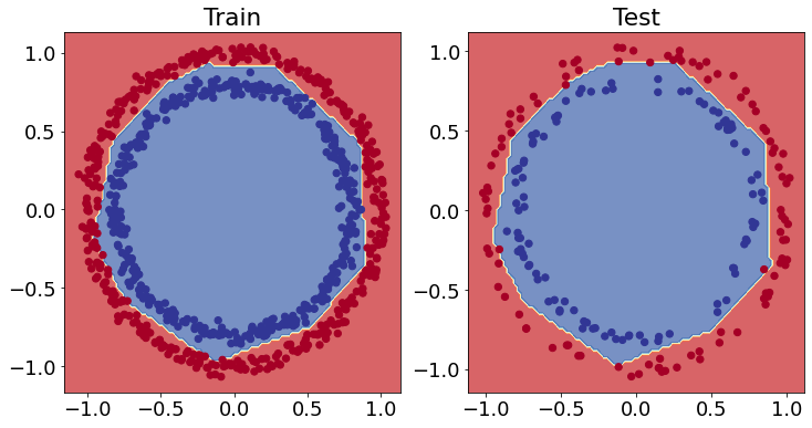
# Plot the decision boundaries for the training and test sets
plt.figure(figsize=(12, 6))
plt.subplot(1, 2, 1)
plt.title("Train")
plot_decision_boundary(model_3, X=X_train, y=y_train)
plt.subplot(1, 2, 2)
plt.title("Test")
plot_decision_boundary(model_3, X=X_test, y=y_test)
plt.show()

doing binary classifcation...
doing binary classifcation...

png

NOx classification example

data = pd.read_csv('https://raw.githubusercontent.com/arminnorouzi/ML-developed_course/main/Data/Engine_NOx_classification.csv')
data.head()

	Load [ft.lb]	Engine speed [rpm]	mf [mg/stroke]	Pr [PSI]	NOx [ppm]
0	50	2502.400000	31.222326	15285.16744	103.899724
1	50	2248.666667	30.116667	15155.13333	112.610181
2	75	2502.000000	38.300000	15356.00000	114.789893
3	100	2504.000000	42.900000	15296.00000	125.411970
4	75	2262.000000	34.100000	15254.00000	126.524679

cdf = data[['Load [ft.lb]','Engine speed [rpm]','mf [mg/stroke]','Pr [PSI]', 'High NOx']]

msk = np.random.rand(len(data)) < 0.8
train = cdf[msk]
test = cdf[~msk]

Plot training data then test data

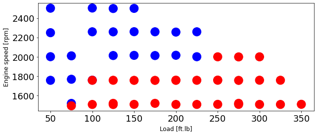
colors = {0: 'blue', 1:'red', 2:'green', 3:'coral', 4:'orange', 5:'black'}

area = 300
# area = 200
plt.figure(1, figsize=(10, 4))
plt.scatter(train['Load [ft.lb]'], train['Engine speed [rpm]'], s=area, c=np.array(train['High NOx'].map(colors).tolist()), alpha=1)

plt.xlabel('Load [ft.lb]', fontsize=12)
plt.ylabel('Engine speed [rpm]', fontsize=12)

Text(0, 0.5, 'Engine speed [rpm]')

png

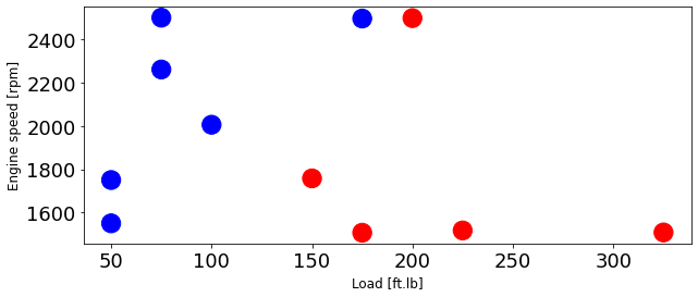
area = 300
# area = 200
plt.figure(1, figsize=(10, 4))
plt.scatter(test['Load [ft.lb]'], test['Engine speed [rpm]'], s=area, c=np.array(test['High NOx'].map(colors).tolist()), alpha=1)

plt.xlabel('Load [ft.lb]', fontsize=12)
plt.ylabel('Engine speed [rpm]', fontsize=12)

Text(0, 0.5, 'Engine speed [rpm]')

png

Scaling inputs

from sklearn import preprocessing


train_x = np.asanyarray(train[['Load [ft.lb]','Engine speed [rpm]']])
train_y = np.asanyarray(train[['High NOx']])

test_x = np.asanyarray(test[['Load [ft.lb]','Engine speed [rpm]']])
test_y = np.asanyarray(test[['High NOx']])


min_max_scaler = preprocessing.MinMaxScaler()
X_train_minmax = min_max_scaler.fit_transform(train_x)
X_test_minmax = min_max_scaler.transform(test_x)

Building model

# Let's try with sigmoid activation function

# Set random seed
tf.random.set_seed(42)

# Create a model
model_nox = tf.keras.Sequential([
  tf.keras.layers.Dense(2, activation="relu", name ="Input_Layer"), # hidden layer 1, ReLU activation
  tf.keras.layers.Dense(5, activation="relu", name ="Hidden_layer_1"), # hidden layer 2, ReLU activation
  tf.keras.layers.Dense(1, activation="sigmoid", name ="Output_Layer") # ouput layer, sigmoid activation
], name = "My_NN_classification_model")

# Compile the model
model_nox.compile(loss=tf.keras.losses.binary_crossentropy,
                optimizer=tf.keras.optimizers.Adam(learning_rate=0.01),
                metrics=['accuracy'])



# Fit the model
history = model_nox.fit(X_train_minmax, train_y, epochs=1000, verbose=0)

model_nox.summary()


plt.figure(figsize=(10,10))
plt.subplot(2, 1, 1)
plt.plot(history.history['loss'])
plt.title("loss")
plt.subplot(2, 1, 2)
plt.plot(history.history['accuracy'])
plt.title("accuracy")
plt.show()

Model: "My_NN_classification_model"
_________________________________________________________________
 Layer (type)                Output Shape              Param #
=================================================================
 Input_Layer (Dense)         (None, 2)                 6

 Hidden_layer_1 (Dense)      (None, 5)                 15

 Output_Layer (Dense)        (None, 1)                 6

=================================================================
Total params: 27
Trainable params: 27
Non-trainable params: 0
_________________________________________________________________

png

# Plot the decision boundaries for the training and test sets
plt.figure(figsize=(12, 6))
plt.subplot(1, 2, 1)
plt.title("Train")
plot_decision_boundary(model_nox, X=X_train_minmax, y=train_y)
plt.subplot(1, 2, 2)
plt.title("Test")
plot_decision_boundary(model_nox, X=X_test_minmax, y=test_y)
plt.show()

doing binary classifcation...
doing binary classifcation...

png

Improving model

Need to add compelxity: Add more hidden unit or layer
adding L2 regularization to avoid overfitting
increase max epochs

# Let's try with sigmoid activation function

# Set random seed
tf.random.set_seed(42)

# Create a model
model_nox = tf.keras.Sequential([
  tf.keras.layers.Dense(4, activation="relu", name ="Input_Layer"), # hidden layer 1, ReLU activation
  tf.keras.layers.Dense(12, activation="relu", name ="Hidden_layer_1", activity_regularizer=tf.keras.regularizers.L2(0.1)), # hidden layer 2, ReLU activation
  tf.keras.layers.Dense(1, activation="sigmoid", name ="Output_Layer") # ouput layer, sigmoid activation
], name = "My_NN_classification_model")

# Compile the model
model_nox.compile(loss=tf.keras.losses.binary_crossentropy,
                optimizer=tf.keras.optimizers.Adam(learning_rate=0.01),
                metrics=['accuracy'])



# Fit the model
history = model_nox.fit(X_train_minmax, train_y, epochs=3000, verbose=0)

model_nox.summary()


plt.figure(figsize=(10,10))
plt.subplot(2, 1, 1)
plt.plot(history.history['loss'])
plt.title("loss")
plt.subplot(2, 1, 2)
plt.plot(history.history['accuracy'])
plt.title("accuracy")
plt.show()

Model: "My_NN_classification_model"
_________________________________________________________________
 Layer (type)                Output Shape              Param #
=================================================================
 Input_Layer (Dense)         (None, 4)                 12

 Hidden_layer_1 (Dense)      (None, 12)                60

 Output_Layer (Dense)        (None, 1)                 13

=================================================================
Total params: 85
Trainable params: 85
Non-trainable params: 0
_________________________________________________________________

png

# Plot the decision boundaries for the training and test sets
plt.figure(figsize=(12, 6))
plt.subplot(1, 2, 1)
plt.title("Train")
plot_decision_boundary(model_nox, X=X_train_minmax, y=train_y)
plt.subplot(1, 2, 2)
plt.title("Test")
plot_decision_boundary(model_nox, X=X_test_minmax, y=test_y)
plt.show()

doing binary classifcation...
doing binary classifcation...

png

It has improved! What is your suggestion to improve more?

Recurent Neural Network with TensorFlow

The Recurrent Neural Network (RNN)

is structured similar to a feedforward ANN
but has backward connections that are used to handle sequential inputs

Simple RNN input output

The simplest RNN for time step $t$ is shown in the Figure
This recurrent neuron receives both inputs $u(t)$ and output from the previous time step, $y(t-1)$.
The output of the first step is generally initialized as zero.
The structure of RNN can be revealed by unrolling it in time, as shown in Figure (right)
The output of the recurrent neuron at the current time step $t$ is a function of past inputs, so a recurrent neuron can be considered a memory.

Simple RNN state and output

Generally, a cell’s state at time step $t$ is given by $h_{(t)}$ ,
where ``$h$’’ stands for ``hidden’’ Cells states are a function of past states and past inputs: $h_{(t)} = f(h_{(t-1)}, u_{(t)})$.
The output of the network at time step $y(t)$ is a function of
- the past state,
- and the current inputs \cite{geron2019hands}.
For the case shown in Figure, the output of the recurrent layer is equal to the state.

$h_t = \phi(W_u^T u_t + w_h h_{t-1} + b_y)$ $\hat{y}(t) = \phi(W_y^T h_t + b_y)$

where $h_t$ is hidden state (memory cell) of RNN,
$W_u$, $W_h$, and $W_y$ are input, hidden state, and output weights,
$b_h$ and $b_y$ are hidden state and output bias values, respectively.
The main reasons that an RNN is computationally efficient is due to:
- parameter sharing
- network weights ($W_u$, $W_h$, and $W_y$) that are constant for the different time steps.

Long Short-Term Memory (LSTM)

when LSTM is compared to RNN, in LSTM the hidden state is split into two main part:
- $h_{(t)}$ the short-term state, and
- $c_{(t)}$ the long-term state.
As shown in Figure, the long-term state $c_{(t-1)}$ traverses the network from left to right.
1. this state first enters the forget gate where past values are dropped
2. then some values (memories) are added to the input gate to get $c_{t}$
3. so at each time step, some memory is added, and some are dropped, and
4. the current long-term state $c_{(t)}$ is output without further change.

Further, after adding new memory, the long-term state is
- replicated,
- passed into the $\tanh$ function, and
- the output gate filters the result to generate the short-term state $h_{(t)}$ (equals to the cell’s output $y_{(t)}$ for this time step) \cite{geron2019hands}.
LTSM computations are summarized here

\begin{equation} \begin{split} i{(t)} &= \sigma(W{ui}^Tu(t) + W{hi}^T h{(t-1)} + bi)
f{(t)} &= \sigma(W{uf}^Tu(t) + W{hf}^T h{(t-1)} + b_f)
o{(t)} &= \sigma(W{uo}^Tu(t) + W{ho}^T h{(t-1)} + b_o)
g{(t)} &= \tanh(W{ug}^Tu(t) + W{hg}^T h{(t-1)} + b_g)
c{(t)} &= f{(t)} \odot c{(t-1)} + i{(t)} \odot g{(t)}
y{(t)} &= h{(t)} = o{(t)} \odot \tanh(c{(t)})
\end{split} \end{equation}

where $W_{u(f,g,i,o)}$ and $W_{h(f,g,i,o)}$ are the weight matrices of each four layer for their connection to input vector $u_{(t)}$ and then
the previous short-term state $h_{(t)}$
In this equation, $\odot$, is element-wise multiplication
$b_{(f,g,i,o)}$ are the bias terms for each four layer.
all four networks $i{(t)}$, $f{(t)}$, $o{(t)}$, and $g{(t)}$ are fully connected (FC) layer;
so each layer of LSTM has four FC layer weights and biases.

To train an RNN, the technique of unrolling it through time

then simply use regular backpropagation.
This strategy is called backpropagation through time (BPTT).

Recurrent neural networks (RNN) are a class of neural networks that is powerful for modeling sequence data such as time series or natural language.

Schematically, a RNN layer uses a for loop to iterate over the timesteps of a sequence, while maintaining an internal state that encodes information about the timesteps it has seen so far.

The Keras RNN API is designed with a focus on:

Ease of use: the built-in keras.layers.RNN, keras.layers.LSTM, keras.layers.GRU layers enable you to quickly build recurrent models without having to make difficult configuration choices.
Ease of customization: You can also define your own RNN cell layer (the inner part of the for loop) with custom behavior, and use it with the generic keras.layers.RNN layer (the for loop itself). This allows you to quickly prototype different research ideas in a flexible way with minimal code.

Dynamics model using DNN:

import pandas as pd
data = pd.read_csv('https://raw.githubusercontent.com/arminnorouzi/ML-developed_course/main/Data/Transient_data.csv') # You need to edit this directory
data.head()

	time	SOI	FQ	Load
0	0.00	-3.8	24.6	0.001000
1	0.08	-3.8	24.6	123.612898
2	0.16	-3.8	24.6	154.786556
3	0.24	-3.8	24.6	155.228298
4	0.32	-3.8	24.6	155.283862

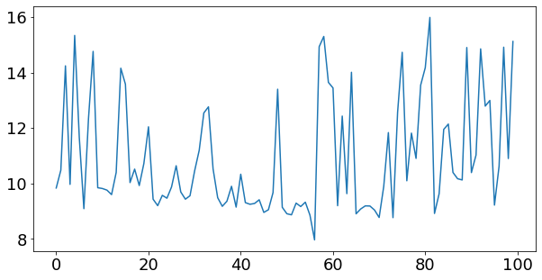
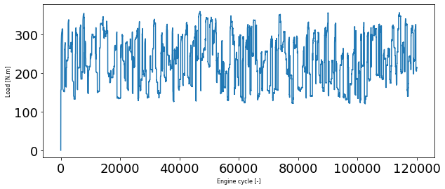
This is a transient data, so we can plot it over time or over each engine cycle (0.08 second)

area = 300
# area = 200
plt.figure(1, figsize=(10, 4))
plt.plot(data['Load'])

plt.xlabel('Engine cycle [-]', fontsize=8)
plt.ylabel('Load [N.m]', fontsize=8)

Text(0, 0.5, 'Load [N.m]')

png

X = np.asanyarray(data[['SOI','FQ']])
Y = np.asanyarray(data[['Load']])
len(X)

# Split data into train and test sets


X_train = X[:90000] # first 90000 cycles (75% of data)
y_train = Y[:90000]

X_test = X[90000:] # last 30000 cycles (25% of data)
y_test = Y[90000:]

len(X_train), len(X_test)

min_max_scaler = preprocessing.MinMaxScaler()
X_train_minmax = min_max_scaler.fit_transform(X_train)
X_test_minmax = min_max_scaler.transform(X_test)

min_max_scaler.data_max_

array([ 2. , 59.7])

min_max_scaler.data_min_

array([-9.9, 20. ])

# Let's try with sigmoid activation function

# Set random seed
tf.random.set_seed(42)

# Create a model
model_load = tf.keras.Sequential([
  tf.keras.layers.InputLayer(input_shape = (X_train_minmax.shape[1], )),
  tf.keras.layers.Dense(32, activation="relu"),
  tf.keras.layers.Dense(16, activation="relu"),
  tf.keras.layers.Dense(1, name ="Output_Layer")
])

# Compile the model
model_load.compile(loss=tf.keras.losses.mse,
                optimizer=tf.keras.optimizers.Adam(learning_rate=0.0001),
                metrics=['mse'])



# Fit the model
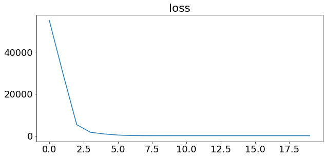
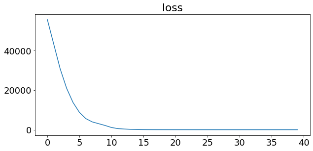
history = model_load.fit(X_train_minmax, y_train, epochs=20, verbose=0)

model_load.summary()


plt.figure(figsize=(10,10))
plt.subplot(2, 1, 1)
plt.plot(history.history['loss'])
plt.title("loss")

Model: "sequential_9"
_________________________________________________________________
 Layer (type)                Output Shape              Param #
=================================================================
 dense_15 (Dense)            (None, 32)                96

 dense_16 (Dense)            (None, 16)                528

 Output_Layer (Dense)        (None, 1)                 17

=================================================================
Total params: 641
Trainable params: 641
Non-trainable params: 0
_________________________________________________________________





Text(0.5, 1.0, 'loss')

png

X_train_minmax.shape, y_train.shape

((90000, 2), (90000, 1))

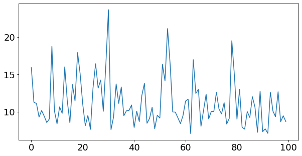
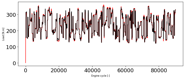
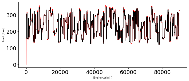
y_train_hat = model_load.predict(X_train_minmax)

plt.figure(1, figsize=(10, 4))
plt.plot(y_train, 'r')
plt.plot(y_train_hat, 'k')

plt.xlabel('Engine cycle [-]', fontsize=8)
plt.ylabel('Load [N.m]', fontsize=8)

Text(0, 0.5, 'Load [N.m]')

png

y_test_hat = model_load.predict(X_test_minmax)

plt.figure(1, figsize=(10, 4))
plt.plot(y_test, 'r')
plt.plot(y_test_hat, 'k')

plt.xlabel('Engine cycle [-]', fontsize=8)
plt.ylabel('Load [N.m]', fontsize=8)

Text(0, 0.5, 'Load [N.m]')

png

Save this model

# Save a model using the HDF5 format
model_load.save("DNNmodel.h5") # note the addition of '.h5' on the end

Dynamics modeling using LSTM layer

As you might’ve guessed, we can also use a recurrent neural network to model our sequential time series data.

Resource: For more on the different types of recurrent neural networks you can use for sequence problems, see the Recurrent Neural Networks section of notebook 08.

one of the most important steps for the LSTM model will be getting our data into the right shape.

The tf.keras.layers.LSTM() layer takes a tensor with [batch, timesteps, feature] dimensions.

The batch dimension gets taken care of for us but our data is currently only has the feature dimension.

To fix this, we can use a tf.keras.layers.Lambda() layer to adjust the shape of our input tensors to the LSTM layer.

from tensorflow.keras import layers

tf.random.set_seed(42)

# Let's build an LSTM model with the Functional API
inputs = layers.Input(shape=(2))
x = layers.Lambda(lambda x: tf.expand_dims(x, axis=1))(inputs) # expand input dimension to be compatible with LSTM
x = layers.LSTM(128, activation='tanh', recurrent_activation='sigmoid', use_bias=True)(x)
output = layers.Dense(1)(x)
model_load_lstm = tf.keras.Model(inputs=inputs, outputs=output)

# Compile model
model_load_lstm.compile(loss=tf.keras.losses.mse,
                optimizer=tf.keras.optimizers.Adam(learning_rate=0.0001),
                metrics=['mse'])

# Seems when saving the model several warnings are appearing: https://github.com/tensorflow/tensorflow/issues/47554
history = model_load_lstm.fit(X_train_minmax, y_train, epochs=40, verbose=0)

model_load_lstm.summary()


plt.figure(figsize=(10,10))
plt.subplot(2, 1, 1)
plt.plot(history.history['loss'])
plt.title("loss")

Model: "model_1"
_________________________________________________________________
 Layer (type)                Output Shape              Param #
=================================================================
 input_4 (InputLayer)        [(None, 2)]               0

 lambda_1 (Lambda)           (None, 1, 2)              0

 lstm_1 (LSTM)               (None, 128)               67072

 dense_17 (Dense)            (None, 1)                 129

=================================================================
Total params: 67,201
Trainable params: 67,201
Non-trainable params: 0
_________________________________________________________________





Text(0.5, 1.0, 'loss')

png

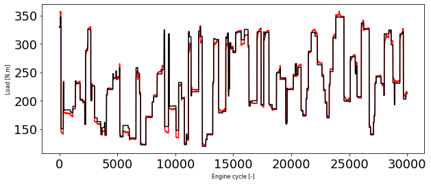
y_train_hat = model_load_lstm.predict(X_train_minmax)

plt.figure(1, figsize=(10, 4))
plt.plot(y_train, 'r')
plt.plot(y_train_hat, 'k')

plt.xlabel('Engine cycle [-]', fontsize=8)
plt.ylabel('Load [N.m]', fontsize=8)

Text(0, 0.5, 'Load [N.m]')

png

y_test_hat = model_load_lstm.predict(X_test_minmax)

plt.figure(1, figsize=(10, 4))
plt.plot(y_test, 'r')
plt.plot(y_test_hat, 'k')

plt.xlabel('Engine cycle [-]', fontsize=8)
plt.ylabel('Load [N.m]', fontsize=8)

Text(0, 0.5, 'Load [N.m]')

png

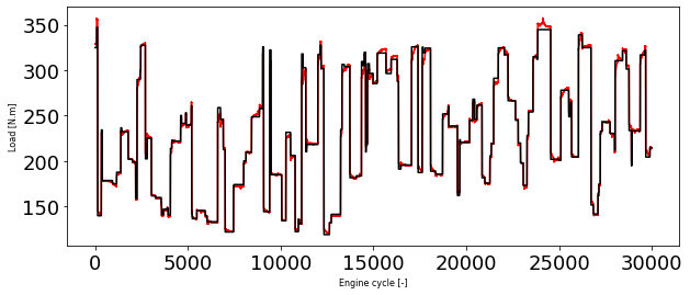
As you can see we have signifiantly better model using LSTM layers

# Save a model using the HDF5 format
model_load_lstm.save("LSTMmodel.h5") # note the addition of '.h5' on the end

Reference

[1] Neural Network Regression with TensorFlow

[2] Neural Network Classification with TensorFlow

[3] Milestone Project 3: Time series forecasting in TensorFlow

[4] Tensorflow Documentation for Python

Share on

Twitter Facebook LinkedIn

Armin Norouzi

Neural Network with TensorFlow

Neural Network with TensorFlow

Neural Network Regression with TensorFlow

Typical architecture of a regresison neural network

Simple regression model

Running experiments to improve a model

Comparing results

Saving a model

Loading a model

Downloading a model (from Google Colab)

Diesel NOx model prediction

Importing data

Improving the mode

Neural Network Classification with TensorFlow

Typical architecture of a classification neural network

Creating data to view and fit

Input and output shapes

Steps in modelling

Evaluating and improving our classification model

NOx classification example

Plot training data then test data

Scaling inputs

Building model

Improving model

Recurent Neural Network with TensorFlow

Dynamics model using DNN:

Dynamics modeling using LSTM layer

Reference

Share on

You May Also Enjoy

Mastering Dynamic Programming: 4 Essential Algorithms for Optimal Solutions

Cracking the Code of Sorting and Searching: 11 Algorithms for Enhanced Efficiency

Mastering Heaps: 5 Essential Algorithms for Optimal Performance

Mastering Linked Lists: 11 Algorithms for Efficient Data Manipulation