Recurrent Neural Networks (RNN) using TensorFlow
Published:
This blog post is a comprehensive guide to Recurrent Neural Networks (RNN) using TensorFlow. The post is compatible with Google Colaboratory and TensorFlow 2.8.2. The objective of the post is to provide readers with a better understanding of RNNs and their applications in time series estimation. The post covers a range of topics related to RNNs, starting with linear regression using TensorFlow and basic neural network modeling. The author then progresses to more advanced ANN models for regression and classification.
The post is compatible with Google Colaboratory and can be accessed through this link:
![]()
Recurrent Neural Networks (RNN) using TensorFlow
- Developed by Armin Norouzi
Compatible with Google Colaboratory- Tensorflow 2.8.2
- Objective: Time series estimation
Table of content:
- Linear Regression with TensorFlow
- Neural Network Basic Modeling using TensorFlow
- Adavnced ANN Model for Regression
- Adavnced ANN Model for Classification
Introduction: What is a time series problem?
What is a time series problem?
Time series problems deal with data over time. Such as, the number of staff members in a company over 10-years, sales of computers for the past 5-years, electricity usage for the past 50-years.
The timeline can be short (seconds/minutes) or long (years/decades). And the problems you might investigate using can usually be broken down into two categories:
| Problem Type | Examples | Output |
|---|---|---|
| Classification | Anomaly detection, time series identification (where did this time series come from?) | Discrete (a label) |
| Forecasting | Predicting stock market prices, forecasting future demand for a product, stocking inventory requirements | Continuous (a number) |
In both cases above, a supervised learning approach is often used. Meaning, you would have some example data and a label assosciated with that data.
# Check for GPU
!nvidia-smi -L
GPU 0: Tesla P100-PCIE-16GB (UUID: GPU-fdfc7a94-b419-68c4-6867-5bb173c97592)
Load and prepare data
Download data
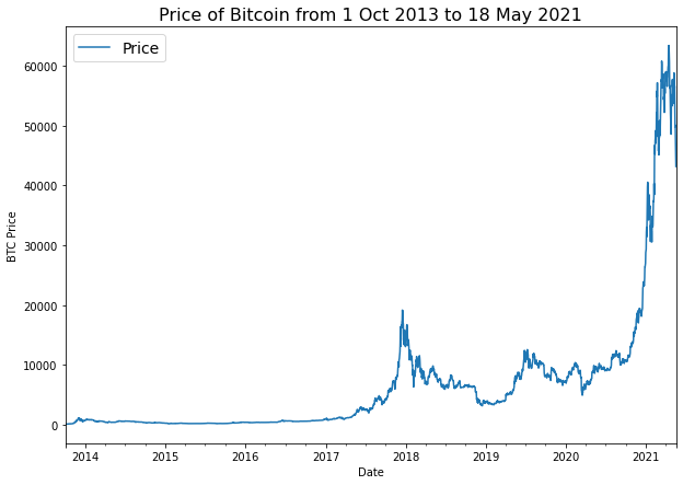
To build a time series forecasting model, price of Bitcoin from from 01 October 2013 to 18 May 2021 will be used. The original data source is Coindesk page for Bitcoin prices.
# Turn .csv files into pandas DataFrame's
import pandas as pd
df = pd.read_csv("https://raw.githubusercontent.com/arminnorouzi/machine_learning_course_UofA_MECE610/main/Data/bitcoin_price.csv",
                 parse_dates=["Date"],
                 index_col=["Date"]) # parse the date column (tell pandas column 1 is a datetime)
df.head()
| Currency | Closing Price (USD) | 24h Open (USD) | 24h High (USD) | 24h Low (USD) | |
|---|---|---|---|---|---|
| Date | |||||
| 2013-10-01 | BTC | 123.65499 | 124.30466 | 124.75166 | 122.56349 |
| 2013-10-02 | BTC | 125.45500 | 123.65499 | 125.75850 | 123.63383 |
| 2013-10-03 | BTC | 108.58483 | 125.45500 | 125.66566 | 83.32833 |
| 2013-10-04 | BTC | 118.67466 | 108.58483 | 118.67500 | 107.05816 |
| 2013-10-05 | BTC | 121.33866 | 118.67466 | 121.93633 | 118.00566 |
print(f"size of dataset = {len(df)}")
size of dataset = 2787
This data set is historical price of Bitcoin for the past ~8 years but there is only 2787 total samples. This is something we have with time series data. Often, the number of samples is not as large as other kinds of data.
For example, collecting one sample at different time frames results in:
| 1 sample per timeframe | Number of samples per year |
|---|---|
| Second | 31,536,000 |
| Hour | 8,760 |
| Day | 365 |
| Week | 52 |
| Month | 12 |
The frequency at which a time series value is collected is often referred to as seasonality. This is usually mesaured in number of samples per year. For example, collecting the price of Bitcoin once per day would result in a time series with a seasonality of 365. Time series data collected with different seasonality values often exhibit seasonal patterns (e.g. electricity demand behing higher in Summer months for air conditioning than Winter months).
Deep learning algorithms usually flourish with lots of data, in the range of thousands to millions of samples.
In our case, we access to the daily prices of Bitcoin, a max of 365 samples per year.
To simplify, let’s remove some of the columns from our data so we will only left with a date index and the closing price.
# Only want closing price for each day
bitcoin_prices = pd.DataFrame(df["Closing Price (USD)"]).rename(columns={"Closing Price (USD)": "Price"})
bitcoin_prices.head()
| Price | |
|---|---|
| Date | |
| 2013-10-01 | 123.65499 |
| 2013-10-02 | 125.45500 |
| 2013-10-03 | 108.58483 |
| 2013-10-04 | 118.67466 |
| 2013-10-05 | 121.33866 |
import matplotlib.pyplot as plt
bitcoin_prices.plot(figsize=(10, 7))
plt.ylabel("BTC Price")
plt.title("Price of Bitcoin from 1 Oct 2013 to 18 May 2021", fontsize=16)
plt.legend(fontsize=14);
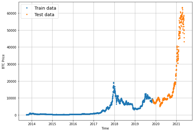
Split train and test data
There is no way we can actually access data from the future.
But we can engineer our test set to be in the future with respect to the training set.
To do this, we can create an abitrary point in time to split our data.
Everything before the point in time can be considered the training set and everything after the point in time can be considered the test set.
# Get bitcoin date array
timesteps = bitcoin_prices.index.to_numpy()
prices = bitcoin_prices["Price"].to_numpy()

timesteps[:10], prices[:10]
(array(['2013-10-01T00:00:00.000000000', '2013-10-02T00:00:00.000000000',
        '2013-10-03T00:00:00.000000000', '2013-10-04T00:00:00.000000000',
        '2013-10-05T00:00:00.000000000', '2013-10-06T00:00:00.000000000',
        '2013-10-07T00:00:00.000000000', '2013-10-08T00:00:00.000000000',
        '2013-10-09T00:00:00.000000000', '2013-10-10T00:00:00.000000000'],
       dtype='datetime64[ns]'),
 array([123.65499, 125.455  , 108.58483, 118.67466, 121.33866, 120.65533,
        121.795  , 123.033  , 124.049  , 125.96116]))
# Create train and test splits the right way for time series data
split_size = int(0.8 * len(prices)) # 80% train, 20% test

# Create train data splits (everything before the split)
X_train, y_train = timesteps[:split_size], prices[:split_size]

# Create test data splits (everything after the split)
X_test, y_test = timesteps[split_size:], prices[split_size:]

print(f"Training feature size = {len(X_train)}")
print(f"Training label size = {len(y_train)}")

print(f"Testing feature size = {len(X_test)}")
print(f"Testing label size = {len(y_test)}")
Training feature size = 2229
Training label size = 2229
Testing feature size = 558
Testing label size = 558
Let’s write a function for plotting time series as we are going to plot a lot of time series:
# Create a function to plot time series data
def plot_time_series(timesteps, values, format='.', start=0, end=None, label=None):
  """
  Plots a timesteps (a series of points in time) against values (a series of values across timesteps).

  Parameters
  ---------
  timesteps : array of timesteps
  values : array of values across time
  format : style of plot, default "."
  start : where to start the plot (setting a value will index from start of timesteps & values)
  end : where to end the plot (setting a value will index from end of timesteps & values)
  label : label to show on plot of values
  """
  # Plot the series
  plt.plot(timesteps[start:end], values[start:end], format, label=label)
  plt.xlabel("Time")
  plt.ylabel("BTC Price")
  if label:
    plt.legend(fontsize=14) # make label bigger
  plt.grid(True)
# Try out our plotting function
plt.figure(figsize=(10, 7))
plot_time_series(timesteps=X_train, values=y_train, label="Train data")
plot_time_series(timesteps=X_test, values=y_test, label="Test data")
Windowing dataset
Windowing is a method to turn a time series dataset into supervised learning problem.
In other words, we want to use windows of the past to predict the future.
For example for a univariate time series, windowing for one week (window=7) to predict the next single value (horizon=1) might look like:
Window for one week (univariate time series)

[0, 1, 2, 3, 4, 5, 6] -> [7]
[1, 2, 3, 4, 5, 6, 7] -> [8]
[2, 3, 4, 5, 6, 7, 8] -> [9]
Or for the price of Bitcoin, it will look like:
Window for one week with the target of predicting the next day (Bitcoin prices)

[123.654, 125.455, 108.584, 118.674, 121.338, 120.655, 121.795] -> [123.033]
[125.455, 108.584, 118.674, 121.338, 120.655, 121.795, 123.033] -> [124.049]
[108.584, 118.674, 121.338, 120.655, 121.795, 123.033, 124.049] -> [125.961]
#  these are testing value for checking function and will be changed in each model
HORIZON = 1 # predict 1 step at a time
WINDOW_SIZE = 7 # use a week worth of timesteps to predict the horizon
# Create function to label windowed data
def get_labelled_windows(x, horizon=1):
  """
  Creates labels for windowed dataset.

  E.g. if horizon=1 (default)
  Input: [1, 2, 3, 4, 5, 6] -> Output: ([1, 2, 3, 4, 5], [6])
  """
  return x[:, :-horizon], x[:, -horizon:]
import tensorflow as tf

# Test out the window labelling function
test_window, test_label = get_labelled_windows(tf.expand_dims(tf.range(8)+1, axis=0), horizon=HORIZON)
print(f"Window: {tf.squeeze(test_window).numpy()} -> Label: {tf.squeeze(test_label).numpy()}")
Window: [1 2 3 4 5 6 7] -> Label: 8
Now we need a way to make windows for an entire time series.
We could do this with Python for loops, however, for large time series, that’d be quite slow.
To speed things up, we will leverage NumPy’s array indexing.
Let’s write a function which:
- Creates a window step of specific window size, for example:
[[0, 1, 2, 3, 4, 5, 6, 7]] - Uses NumPy indexing to create a 2D of multiple window steps, for example:
[[0, 1, 2, 3, 4, 5, 6, 7],
 [1, 2, 3, 4, 5, 6, 7, 8],
 [2, 3, 4, 5, 6, 7, 8, 9]]
- Uses the 2D array of multuple window steps to index on a target series
- Uses the
get_labelled_windows()function we created above to turn the window steps into windows with a specified horizon
Resource: The function created below has been adapted from Syafiq Kamarul Azman’s article Fast and Robust Sliding Window Vectorization with NumPy.
import numpy as np

# Create function to view NumPy arrays as windows
def make_windows(x, window_size=7, horizon=1):
  """
  Turns a 1D array into a 2D array of sequential windows of window_size.
  """
  # 1. Create a window of specific window_size (add the horizon on the end for later labelling)
  window_step = np.expand_dims(np.arange(window_size+horizon), axis=0)
  # print(f"Window step:\n {window_step}")

  # 2. Create a 2D array of multiple window steps (minus 1 to account for 0 indexing)
  window_indexes = window_step + np.expand_dims(np.arange(len(x)-(window_size+horizon-1)), axis=0).T # create 2D array of windows of size window_size
  # print(f"Window indexes:\n {window_indexes[:3], window_indexes[-3:], window_indexes.shape}")

  # 3. Index on the target array (time series) with 2D array of multiple window steps
  windowed_array = x[window_indexes]

  # 4. Get the labelled windows
  windows, labels = get_labelled_windows(windowed_array, horizon=horizon)

  return windows, labels
full_windows, full_labels = make_windows(prices, window_size=WINDOW_SIZE, horizon=HORIZON)
len(full_windows), len(full_labels)
(2780, 2780)
# View the first 3 windows/labels
for i in range(10):
  print(f"Window: {full_windows[i]} -> Label: {full_labels[i]}")
Window: [123.65499 125.455   108.58483 118.67466 121.33866 120.65533 121.795  ] -> Label: [123.033]
Window: [125.455   108.58483 118.67466 121.33866 120.65533 121.795   123.033  ] -> Label: [124.049]
Window: [108.58483 118.67466 121.33866 120.65533 121.795   123.033   124.049  ] -> Label: [125.96116]
Window: [118.67466 121.33866 120.65533 121.795   123.033   124.049   125.96116] -> Label: [125.27966]
Window: [121.33866 120.65533 121.795   123.033   124.049   125.96116 125.27966] -> Label: [125.9275]
Window: [120.65533 121.795   123.033   124.049   125.96116 125.27966 125.9275 ] -> Label: [126.38333]
Window: [121.795   123.033   124.049   125.96116 125.27966 125.9275  126.38333] -> Label: [135.24199]
Window: [123.033   124.049   125.96116 125.27966 125.9275  126.38333 135.24199] -> Label: [133.20333]
Window: [124.049   125.96116 125.27966 125.9275  126.38333 135.24199 133.20333] -> Label: [142.76333]
Window: [125.96116 125.27966 125.9275  126.38333 135.24199 133.20333 142.76333] -> Label: [137.92333]
You can find a function which achieves similar results to the ones we implemented above at tf.keras.preprocessing.timeseries_dataset_from_array(). Just like ours, it takes in an array and returns a windowed dataset. It has the benefit of returning data in the form of a tf.data.Dataset instance (we’ll see how to do this with our own data later).
Turning windows into training and test sets
# Make the train/test splits
def make_train_test_splits(windows, labels, test_split=0.2):
  """
  Splits matching pairs of windows and labels into train and test splits.
  """
  split_size = int(len(windows) * (1-test_split)) # this will default to 80% train/20% test
  train_windows = windows[:split_size]
  train_labels = labels[:split_size]
  test_windows = windows[split_size:]
  test_labels = labels[split_size:]
  return train_windows, test_windows, train_labels, test_labels
train_windows, test_windows, train_labels, test_labels = make_train_test_splits(full_windows, full_labels)
len(train_windows), len(test_windows), len(train_labels), len(test_labels)
(2224, 556, 2224, 556)
train_windows[:5], train_labels[:5]
(array([[123.65499, 125.455  , 108.58483, 118.67466, 121.33866, 120.65533,
         121.795  ],
        [125.455  , 108.58483, 118.67466, 121.33866, 120.65533, 121.795  ,
         123.033  ],
        [108.58483, 118.67466, 121.33866, 120.65533, 121.795  , 123.033  ,
         124.049  ],
        [118.67466, 121.33866, 120.65533, 121.795  , 123.033  , 124.049  ,
         125.96116],
        [121.33866, 120.65533, 121.795  , 123.033  , 124.049  , 125.96116,
         125.27966]]), array([[123.033  ],
        [124.049  ],
        [125.96116],
        [125.27966],
        [125.9275 ]]))
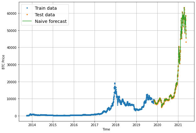
Base Line Modeling: Model 0 - Naïve forecast (baseline)
One of the most common baseline models for time series forecasting, the naïve model (also called the naïve forecast), requires no training at all.
That’s because all the naïve model does is use the previous timestep value to predict the next timestep value.
The formula looks like this:
\[\hat{y}_{t} = y_{t-1}\]The prediction at timestep t (y-hat) is equal to the value at timestep t-1 (the previous timestep).
In an open system (like a stock market or crypto market), you will often find beating the naïve forecast with any kind of model is quite hard.
Note: For the sake of this notebook, an open system is a system where inputs and outputs can freely flow, such as a market (stock or crypto). Where as, a closed system the inputs and outputs are contained within the system (like a poker game with your buddies, you know the buy in and you know how much the winner can get). Time series forecasting in open systems is generally quite poor.
# Create a naïve forecast
naive_forecast = []
for i in range(1,len(y_test)):
  naive_forecast.append(y_test[i - 1])
naive_forecast[:10], naive_forecast[-10:] # View frist 10 and last 10
([9226.4858208826,
  8794.3586445233,
  8798.0420546256,
  9081.1868784913,
  8711.5343391679,
  8760.8927181435,
  8749.520591019,
  8656.970922354,
  8500.6435581622,
  8469.2608988992],
 [57107.1206718864,
  58788.2096789273,
  58102.1914262342,
  55715.5466512869,
  56573.5554719043,
  52147.8211869823,
  49764.1320815975,
  50032.6931367648,
  47885.6252547166,
  45604.6157536131])
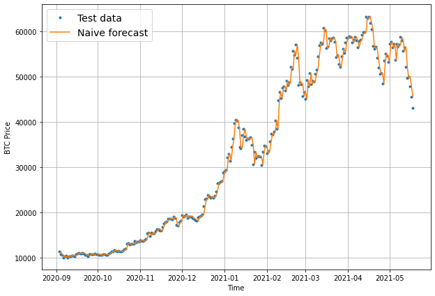
# Plot naive forecast
plt.figure(figsize=(10, 7))
plot_time_series(timesteps=X_train, values=y_train, label="Train data")
plot_time_series(timesteps=X_test, values=y_test, label="Test data")
plot_time_series(timesteps=X_test[1:], values=naive_forecast, format="-", label="Naive forecast");
plt.figure(figsize=(10, 7))
offset = 300 # offset the values by 300 timesteps
plot_time_series(timesteps=X_test, values=y_test, start=offset, label="Test data")
plot_time_series(timesteps=X_test[1:], values=naive_forecast, format="-", start=offset, label="Naive forecast");
Evaluating a time series model
- Scale-dependent errors
These are metrics which can be used to compare time series values and forecasts that are on the same scale.
For example, Bitcoin historical prices in USD veresus Bitcoin forecast values in USD.
| Metric | Details | Code |
|---|---|---|
| MAE (mean absolute error) | Easy to interpret (a forecast is X amount different from actual amount). Forecast methods which minimises the MAE will lead to forecasts of the median. | tf.keras.metrics.mean_absolute_error() |
| RMSE (root mean square error) | Forecasts which minimise the RMSE lead to forecasts of the mean. | tf.sqrt(tf.keras.metrics.mean_square_error()) |
- Percentage errors
Percentage errors do not have units, this means they can be used to compare forecasts across different datasets.
| Metric | Details | Code |
|---|---|---|
| MAPE (mean absolute percentage error) | Most commonly used percentage error. May explode (not work) if y=0. | tf.keras.metrics.mean_absolute_percentage_error() |
| sMAPE (symmetric mean absolute percentage error) | Recommended not to be used by Forecasting: Principles and Practice, though it is used in forecasting competitions. | Custom implementation |
- Scaled errors
Scaled errors are an alternative to percentage errors when comparing forecast performance across different time series.
| Metric | Details | Code |
|---|---|---|
| MASE (mean absolute scaled error). | MASE equals one for the naive forecast (or very close to one). A forecast which performs better than the naïve should get <1 MASE. | See sktime’s mase_loss() |
# Let's get TensorFlow!
import tensorflow as tf
# MASE implemented courtesy of sktime - https://github.com/alan-turing-institute/sktime/blob/ee7a06843a44f4aaec7582d847e36073a9ab0566/sktime/performance_metrics/forecasting/_functions.py#L16
def mean_absolute_scaled_error(y_true, y_pred):
  """
  Implement MASE (assuming no seasonality of data).
  """
  mae = tf.reduce_mean(tf.abs(y_true - y_pred))

  # Find MAE of naive forecast (no seasonality)
  mae_naive_no_season = tf.reduce_mean(tf.abs(y_true[1:] - y_true[:-1])) # our seasonality is 1 day (hence the shifting of 1 day)

  return mae / mae_naive_no_season
You will notice the version of MASE above doesn’t take in the training values like sktime’s mae_loss(). In our case, we are comparing the MAE of our predictions on the test to the MAE of the naïve forecast on the test set.
In practice, if we have created the function correctly, the naïve model should achieve an MASE of 1 (or very close to 1). Any model worse than the naïve forecast will achieve an MASE of >1 and any model better than the naïve forecast will achieve an MASE of <1.
Let’s put each of our different evaluation metrics together into a function.
def evaluate_preds(y_true, y_pred):
  # Make sure float32 (for metric calculations)
  y_true = tf.cast(y_true, dtype=tf.float32)
  y_pred = tf.cast(y_pred, dtype=tf.float32)

  # Calculate various metrics
  mae = tf.keras.metrics.mean_absolute_error(y_true, y_pred)
  mse = tf.keras.metrics.mean_squared_error(y_true, y_pred) # puts and emphasis on outliers (all errors get squared)
  rmse = tf.sqrt(mse)
  mape = tf.keras.metrics.mean_absolute_percentage_error(y_true, y_pred)
  mase = mean_absolute_scaled_error(y_true, y_pred)

  res = {"mae": mae.numpy(),
          "mse": mse.numpy(),
          "rmse": rmse.numpy(),
          "mape": mape.numpy(),
          "mase": mase.numpy()}

  print("MAE = ", round(res['mae'], 2))
  print("MSE = ", round(res['mse'], 2))
  print("RMSE = ", round(res['rmse'], 2))
  print("MAPE = ", round(res['mape'], 2))
  print("MASE = ", round(res['mase'], 2))
  return res
How about we test our function on the naive forecast?
naive_results = evaluate_preds(y_true=y_test[1:],
                               y_pred=naive_forecast)
MAE =  567.98
MSE =  1147547.0
RMSE =  1071.24
MAPE =  2.52
MASE =  1.0
Taking a look at the naïve forecast’s MAE, it seems on average each forecast is ~$567 different than the actual Bitcoin price.
How does this compare to the average price of Bitcoin in the test dataset?
# Find average price of Bitcoin in test dataset
round(tf.reduce_mean(y_test).numpy(), 2)
20056.63
Okay, looking at these two values is starting to give us an idea of how our model is performing:
The average price of Bitcoin in the test dataset is: $20,056 (note: average may not be the best measure here, since the highest price is over 3x this value and the lowest price is over 4x lower)
Each prediction in naive forecast is on average off by: $567
Is this enough to say it’s a good model?
Alternative baseline models
There are many other kinds of models you may want to look into for building baselines/performing forecasts:
| Model/Library Name | Resource |
|---|---|
| Moving average | https://machinelearningmastery.com/moving-average-smoothing-for-time-series-forecasting-python/ |
| ARIMA (Autoregression Integrated Moving Average) | https://machinelearningmastery.com/arima-for-time-series-forecasting-with-python/ |
| sktime (Scikit-Learn for time series) | https://github.com/alan-turing-institute/sktime |
| TensorFlow Decision Forests (random forest, gradient boosting trees) | https://www.tensorflow.org/decision_forests |
| Facebook Kats (purpose-built forecasting and time series analysis library by Facebook) | https://github.com/facebookresearch/Kats |
| LinkedIn Greykite (flexible, intuitive and fast forecasts) | https://github.com/linkedin/greykite |
Modeling
There are two important terms in time series estimation:
- horizon = number of timesteps to predict into future
- window = number of timesteps from past used to predict horizon
For example, if we wanted to predict the price of Bitcoin for tomorrow (1 day in the future) using the previous week’s worth of Bitcoin prices (7 days in the past), the horizon would be 1 and the window would be 7.
Now, how about those modelling experiments?
| Model Number | Model Type | Horizon size | Window size | Extra data |
|---|---|---|---|---|
| 1 | Dense model | 1 | 7 | NA |
| 2 | Dense model | 1 | 30 | NA |
| 3 | Dense model | 7 | 30 | NA |
| 4 | Conv1D | 1 | 7 | NA |
| 5 | LSTM | 1 | 7 | NA |
| 6 | Dense model with multivariate data | 1 | 7 | Block reward size |
| 7 | N-BEATs Algorithm | 1 | 7 | NA |
| 8 | Future prediction model (model to predict future values) | 1 | 7 | NA |
Making a modelling checkpoint
Because our model’s performance will fluctuate from experiment to experiment, we’ll want to make sure we’re comparing apples to apples.
For example, if model_1 performed incredibly well on epoch 55 but its performance fell off toward epoch 100, we want the version of the model from epoch 55 to compare to other models rather than the version of the model from epoch 100.
To take of this, we will implement a ModelCheckpoint callback.
The ModelCheckpoint callback will monitor our model’s performance during training and save the best model to file by setting save_best_only=True.
That way when evaluating our model we could restore its best performing configuration from file.
import os

# Create a function to implement a ModelCheckpoint callback with a specific filename
def create_model_checkpoint(model_name, save_path="model_experiments"):
  return tf.keras.callbacks.ModelCheckpoint(filepath=os.path.join(save_path, model_name), # create filepath to save model
                                            verbose=0, # only output a limited amount of text
                                            save_best_only=True) # save only the best model to file
Model 1: Dense model (window = 7, horizon = 1)
model_1 will have:
- A single dense layer with 128 hidden units and ReLU (rectified linear unit) activation
- An output layer with linear activation (or no activation) Adam optimizer and MAE loss function
- Batch size of 128
- 100 epochs
import tensorflow as tf
from tensorflow.keras import layers
# Set random seed for as reproducible results as possible
tf.random.set_seed(42)
# Construct model
model_1 = tf.keras.Sequential([
layers.Dense(128, activation="relu"),
layers.Dense(HORIZON, activation="linear") # linear activation is the same as having no activation
], name="model_1_dense") # give the model a name so we can save it
# Compile model
model_1.compile(loss="mae",
optimizer=tf.keras.optimizers.Adam(),
metrics=["mae"]) # we don't necessarily need this when the loss function is already MAE
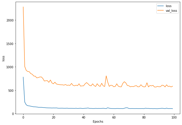
# Fit model
history_1 = model_1.fit(x=train_windows, # train windows of 7 timesteps of Bitcoin prices
y=train_labels, # horizon value of 1 (using the previous 7 timesteps to predict next day)
epochs=100,
verbose=0,
batch_size=128,
validation_data=(test_windows, test_labels),
callbacks=[create_model_checkpoint(model_name=model_1.name)]) # create ModelCheckpoint callback to save best model
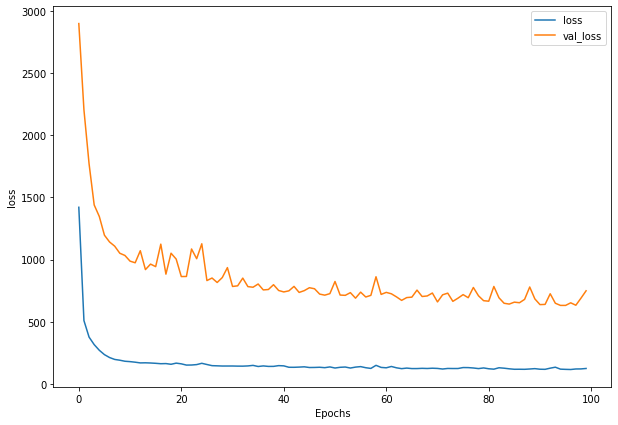
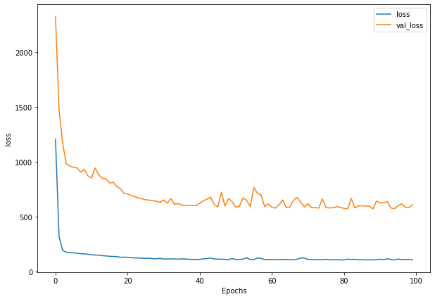
Write a function to plot loss
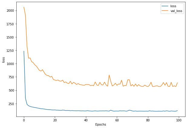
def plot_loss(history):
  plt.figure(figsize=(10, 7))
  plt.plot(history.history['loss'], label = "loss")
  plt.plot(history.history['val_loss'], label= "val_loss")
  plt.xlabel("Epochs")
  plt.ylabel("loss")
  plt.legend()
  plt.show()
plot_loss(history_1)
Write a function to get prediction based on model and input data
def make_preds(model, input_data):
  """
  Uses model to make predictions on input_data.

  Parameters
  ----------
  model: trained model
  input_data: windowed input data (same kind of data model was trained on)

  Returns model predictions on input_data.
  """
  forecast = model.predict(input_data)
  return tf.squeeze(forecast) # return 1D array of predictions
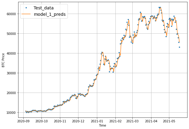
# Make predictions using model_1 on the test dataset and view the results
model_1_preds = make_preds(model_1, test_windows)
len(model_1_preds), model_1_preds[:10]
(556, <tf.Tensor: shape=(10,), dtype=float32, numpy=
 array([8801.184, 8714.926, 8972.654, 8760.343, 8676.047, 8679.056,
        8641.019, 8451.335, 8412.065, 8468.017], dtype=float32)>)
# Evaluate preds
model_1_results = evaluate_preds(y_true=tf.squeeze(test_labels), # reduce to right shape
                                 y_pred=model_1_preds)
MAE =  585.98
MSE =  1197801.1
RMSE =  1094.44
MAPE =  2.61
MASE =  1.03
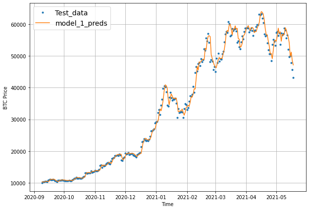
offset = 300
plt.figure(figsize=(10, 7))
# Account for the test_window offset and index into test_labels to ensure correct plotting
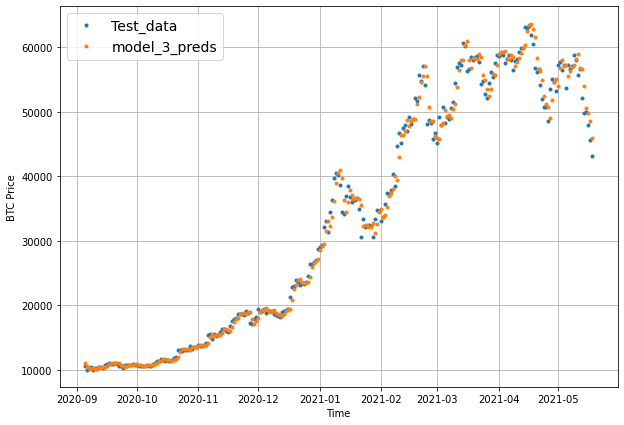
plot_time_series(timesteps=X_test[-len(test_windows):], values=test_labels[:, 0], start=offset, label="Test_data")
plot_time_series(timesteps=X_test[-len(test_windows):], values=model_1_preds, start=offset, format="-", label="model_1_preds")
Model 2: Dense model (window = 30, horizon = 1)
We’ll start our second modelling experiment by preparing datasets using the functions we created earlier.
HORIZON = 1 # predict one step at a time
WINDOW_SIZE = 30 # use 30 timesteps in the past
# Make windowed data with appropriate horizon and window sizes
full_windows, full_labels = make_windows(prices, window_size=WINDOW_SIZE, horizon=HORIZON)
len(full_windows), len(full_labels)
(2757, 2757)
# Make train and testing windows
train_windows, test_windows, train_labels, test_labels = make_train_test_splits(windows=full_windows, labels=full_labels)
len(train_windows), len(test_windows), len(train_labels), len(test_labels)
(2205, 552, 2205, 552)
# Set random seed for as reproducible results as possible
tf.random.set_seed(42)
# Construct model
model_2 = tf.keras.Sequential([
layers.Dense(128, activation="relu"),
layers.Dense(HORIZON, activation="linear") # linear activation is the same as having no activation
], name="model_2_dense") # give the model a name so we can save it
# Compile model
model_2.compile(loss="mae",
optimizer=tf.keras.optimizers.Adam(),
metrics=["mae"]) # we don't necessarily need this when the loss function is already MAE
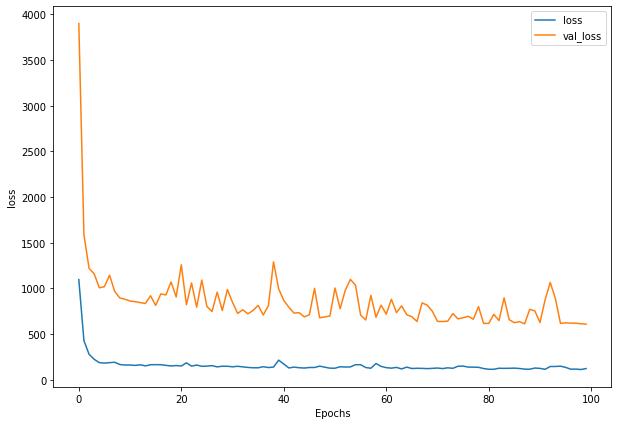
# Fit model
history_2 = model_2.fit(x=train_windows, # train windows of 7 timesteps of Bitcoin prices
y=train_labels, # horizon value of 1 (using the previous 7 timesteps to predict next day)
epochs=100,
verbose=0,
batch_size=128,
validation_data=(test_windows, test_labels),
callbacks=[create_model_checkpoint(model_name=model_2.name)]) # create ModelCheckpoint callback to save best model
plot_loss(history_2)
model_2_preds = make_preds(model_2, test_windows)

# Evaluate preds
model_2_results = evaluate_preds(y_true=tf.squeeze(test_labels), # reduce to right shape
                                 y_pred=model_2_preds)
MAE =  608.96
MSE =  1281440.6
RMSE =  1132.01
MAPE =  2.77
MASE =  1.06
offset = 300
plt.figure(figsize=(10, 7))
# Account for the test_window offset and index into test_labels to ensure correct plotting
plot_time_series(timesteps=X_test[-len(test_windows):], values=test_labels[:, 0], start=offset, label="Test_data")
plot_time_series(timesteps=X_test[-len(test_windows):], values=model_2_preds, start=offset, format="-", label="model_1_preds")
How about we try loading in the best performing model_2 which was saved to file thanks to our ModelCheckpoint callback.
# Load in best performing model
model_2 = tf.keras.models.load_model("model_experiments/model_2_dense/")
model_2.evaluate(test_windows, test_labels)
18/18 [==============================] - 0s 2ms/step - loss: 608.9620 - mae: 608.9620


[608.9619750976562, 608.9619750976562]
model_2_preds = make_preds(model_2, test_windows)

# Evaluate preds
model_2_results = evaluate_preds(y_true=tf.squeeze(test_labels), # reduce to right shape
                                 y_pred=model_2_preds)
MAE =  608.96
MSE =  1281440.6
RMSE =  1132.01
MAPE =  2.77
MASE =  1.06
offset = 300
plt.figure(figsize=(10, 7))
# Account for the test_window offset and index into test_labels to ensure correct plotting
plot_time_series(timesteps=X_test[-len(test_windows):], values=test_labels[:, 0], start=offset, label="Test_data")
plot_time_series(timesteps=X_test[-len(test_windows):], values=model_2_preds, start=offset, format="-", label="model_1_preds")

Model 3: Dense (window = 30, horizon = 7)
HORIZON = 7
WINDOW_SIZE = 30

full_windows, full_labels = make_windows(prices, window_size=WINDOW_SIZE, horizon=HORIZON)
len(full_windows), len(full_labels)
(2751, 2751)
tf.random.set_seed(42)

# Create model (same as model_1 except with different data input size)
model_3 = tf.keras.Sequential([
  layers.Dense(128, activation="relu"),
  layers.Dense(HORIZON)
], name="model_3_dense")

model_3.compile(loss="mae",
                optimizer=tf.keras.optimizers.Adam())

history_3 = model_3.fit(train_windows,
                        train_labels,
                        batch_size=128,
                        epochs=100,
                        verbose=0,
                        validation_data=(test_windows, test_labels),
                        callbacks=[create_model_checkpoint(model_name=model_3.name)])

plot_loss(history_3)
# The predictions are going to be 7 steps at a time (this is the HORIZON size)
model_3_preds = make_preds(model_3,
                           input_data=test_windows)

model_3_preds[:5]
<tf.Tensor: shape=(5, 7), dtype=float32, numpy=
array([[8618.386 , 8883.277 , 8671.608 , 8832.306 , 8475.626 , 8866.536 ,
        8538.664 ],
       [8494.315 , 8936.864 , 8819.273 , 8797.718 , 8329.994 , 8864.983 ,
        8599.303 ],
       [8346.091 , 8713.313 , 8656.231 , 8687.275 , 8357.19  , 8598.28  ,
        8452.361 ],
       [8252.554 , 8453.571 , 8461.956 , 8526.071 , 8270.62  , 8458.072 ,
        8210.957 ],
       [8334.274 , 8471.929 , 8378.202 , 8542.983 , 8130.955 , 8392.386 ,
        8133.8506]], dtype=float32)>
Make our evaluation function work for larger horizons
import numpy as np

def evaluate_preds(y_true, y_pred):
  # Make sure float32 (for metric calculations)
  y_true = tf.cast(y_true, dtype=tf.float32)
  y_pred = tf.cast(y_pred, dtype=tf.float32)

  # Calculate various metrics
  mae = tf.keras.metrics.mean_absolute_error(y_true, y_pred)
  mse = tf.keras.metrics.mean_squared_error(y_true, y_pred)
  rmse = tf.sqrt(mse)
  mape = tf.keras.metrics.mean_absolute_percentage_error(y_true, y_pred)
  mase = mean_absolute_scaled_error(y_true, y_pred)

  # Account for different sized metrics (for longer horizons, reduce to single number)
  if mae.ndim > 0: # if mae isn't already a scalar, reduce it to one by aggregating tensors to mean
    mae = tf.reduce_mean(mae)
    mse = tf.reduce_mean(mse)
    rmse = tf.reduce_mean(rmse)
    mape = tf.reduce_mean(mape)
    mase = tf.reduce_mean(mase)

  res = {"mae": mae.numpy(),
          "mse": mse.numpy(),
          "rmse": rmse.numpy(),
          "mape": mape.numpy(),
          "mase": mase.numpy()}

  print("MAE = ", round(res['mae'], 2))
  print("MSE = ", round(res['mse'], 2))
  print("RMSE = ", round(res['rmse'], 2))
  print("MAPE = ", round(res['mape'], 2))
  print("MASE = ", round(res['mase'], 2))

  return res
# Get model_3 results aggregated to single values
model_3_results = evaluate_preds(y_true=test_labels,
                                 y_pred=model_3_preds)
MAE =  748.78
MSE =  1690645.6
RMSE =  812.75
MAPE =  3.54
MASE =  1.31
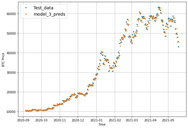
offset = 300
plt.figure(figsize=(10, 7))
plot_time_series(timesteps=X_test[-len(test_windows):], values=test_labels[:, 0], start=offset, label="Test_data")
# Checking the shape of model_3_preds results in [n_test_samples, HORIZON] (this will screw up the plot)
plot_time_series(timesteps=X_test[-len(test_windows):], values=model_3_preds, start=offset, label="model_3_preds")
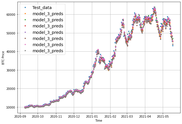
When we try to plot our multi-horizon predicts, we get a funky looking plot.
Again, we can fix this by aggregating our model’s predictions.
Aggregating the predictions (e.g. reducing a 7-day horizon to one value such as the mean) loses information from the original prediction. As in, the model predictions were trained to be made for 7-days but by reducing them to one, we gain the ability to plot them visually but we lose the extra information contained across multiple days.
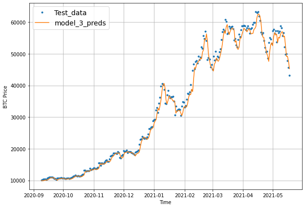
offset = 300
plt.figure(figsize=(10, 7))
# Plot model_3_preds by aggregating them (note: this condenses information so the preds will look fruther ahead than the test data)
plot_time_series(timesteps=X_test[-len(test_windows):],
                 values=test_labels[:, 0],
                 start=offset,
                 label="Test_data")
plot_time_series(timesteps=X_test[-len(test_windows):],
                 values=tf.reduce_mean(model_3_preds, axis=1),
                 format="-",
                 start=offset,
                 label="model_3_preds")
Which of our models is performing best so far? So far, we’ve trained 3 models which use the same architecture but use different data inputs.
Let’s compare them with the naïve model to see which model is performing the best so far.
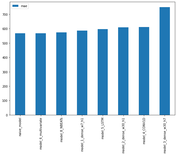
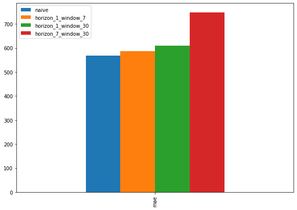
pd.DataFrame({"naive": naive_results["mae"],
              "horizon_1_window_7": model_1_results["mae"],
              "horizon_1_window_30": model_2_results["mae"],
              "horizon_7_window_30": model_3_results["mae"]}, index=["mae"]).plot(figsize=(10, 7), kind="bar");
Model 4: Conv1D
In our case, the input sequence is the previous 7 days of Bitcoin price data and the output is the next day (in seq2seq terms this is called a many to one problem).
Before we build a Conv1D model, let’s recreate our datasets.
HORIZON = 1 # predict next day
WINDOW_SIZE = 7 # use previous week worth of data
# Create windowed dataset
full_windows, full_labels = make_windows(prices, window_size=WINDOW_SIZE, horizon=HORIZON)
len(full_windows), len(full_labels)
(2780, 2780)
# Create train/test splits
train_windows, test_windows, train_labels, test_labels = make_train_test_splits(full_windows, full_labels)
len(train_windows), len(test_windows), len(train_labels), len(test_labels)
(2224, 556, 2224, 556)
Now, since we’re going to be using Conv1D layers, we need to make sure our input shapes are correct.
The Conv1D layer in TensorFlow takes an input of: (batch_size, timesteps, input_dim).
In our case, the batch_size (by default this is 32 but we can change it) is handled for us but the other values will be:
timesteps = WINDOW_SIZE- thetimestepsis also often referred to asfeatures, our features are the previousWINDOW_SIZEvalues of Bitcoininput_dim = HORIZON- our model viewsWINDOW_SIZE(one week) worth of data at a time to predictHORIZON(one day)
Right now, our data has the timesteps dimension ready but we have to adjust it to have the input_dim dimension.
# Check data sample shapes
train_windows[0].shape # returns (WINDOW_SIZE, )
(7,)
To fix this, we could adjust the shape of all of our train_windows or we could use a tf.keras.layers.Lamdba (called a Lambda layer) to do this for us in our model.
tf.random.set_seed(42)

# Create model
model_4 = tf.keras.Sequential([
  # Create Lambda layer to reshape inputs, without this layer, the model will error
  layers.Lambda(lambda x: tf.expand_dims(x, axis=1)), # resize the inputs to adjust for window size / Conv1D 3D input requirements
  layers.Conv1D(filters=128, kernel_size=5, padding="causal", activation="relu"),
  layers.Dense(HORIZON)
], name="model_4_conv1D")

# Compile model
model_4.compile(loss="mae",
                optimizer=tf.keras.optimizers.Adam())
# Fit model
history_4 = model_4.fit(train_windows,
                        train_labels,
                        batch_size=128,
                        epochs=100,
                        verbose=0,
                        validation_data=(test_windows, test_labels),
                        callbacks=[create_model_checkpoint(model_name=model_4.name)])

plot_loss(history_4)
model_4.summary()
Model: "model_4_conv1D"
_________________________________________________________________
 Layer (type)                Output Shape              Param #
=================================================================
 lambda (Lambda)             (None, 1, 7)              0

 conv1d (Conv1D)             (None, 1, 128)            4608

 dense_6 (Dense)             (None, 1, 1)              129

=================================================================
Total params: 4,737
Trainable params: 4,737
Non-trainable params: 0
_________________________________________________________________
# Make predictions
model_4_preds = make_preds(model_4, test_windows)
# Evaluate predictions
model_4_results = evaluate_preds(y_true=tf.squeeze(test_labels),
                                 y_pred=model_4_preds)
MAE =  610.15
MSE =  1242911.1
RMSE =  1114.86
MAPE =  2.76
MASE =  1.07
offset = 300
plt.figure(figsize=(10, 7))
plot_time_series(timesteps=X_test[-len(test_windows):], values=test_labels[:, 0], start=offset, label="Test_data")
# Checking the shape of model_3_preds results in [n_test_samples, HORIZON] (this will screw up the plot)
plot_time_series(timesteps=X_test[-len(test_windows):], values=model_4_preds, start=offset, label="model_3_preds")
Model 5: RNN (LSTM)
Let’s reuse the same data we used for the Conv1D model, except this time we will create an LSTM-cell powered RNN to model our Bitcoin data.
Once again, one of the most important steps for the LSTM model will be getting our data into the right shape.
The tf.keras.layers.LSTM() layer takes a tensor with [batch, timesteps, feature] dimensions.
As mentioned earlier, the batch dimension gets taken care of for us but our data is currently only has the feature dimension (WINDOW_SIZE).
To fix this, just like we did with the Conv1D model, we can use a tf.keras.layers.Lambda() layer to adjust the shape of our input tensors to the LSTM layer.
tf.random.set_seed(42)
# Let's build an LSTM model with the Functional API
inputs = layers.Input(shape=(WINDOW_SIZE))
x = layers.Lambda(lambda x: tf.expand_dims(x, axis=1))(inputs) # expand input dimension to be compatible with LSTM
# print(x.shape)
# x = layers.LSTM(128, activation="relu", return_sequences=True)(x) # this layer will error if the inputs are not the right shape
x = layers.LSTM(128, activation="relu")(x) # using the tanh loss function results in a massive error
# print(x.shape)
# Add another optional dense layer (you could add more of these to see if they improve model performance)
# x = layers.Dense(32, activation="relu")(x)
output = layers.Dense(HORIZON)(x)
model_5 = tf.keras.Model(inputs=inputs, outputs=output, name="model_5_RNN_lstm")
# Compile model
model_5.compile(loss="mae",
optimizer=tf.keras.optimizers.Adam())
# Seems when saving the model several warnings are appearing: https://github.com/tensorflow/tensorflow/issues/47554
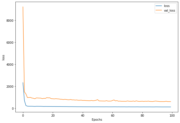
history_5 = model_5.fit(train_windows,
train_labels,
epochs=100,
verbose=0,
batch_size=128,
validation_data=(test_windows, test_labels),
callbacks=[create_model_checkpoint(model_name=model_5.name)])
plot_loss(history_5)
WARNING:tensorflow:Layer lstm will not use cuDNN kernels since it doesn't meet the criteria. It will use a generic GPU kernel as fallback when running on GPU.
WARNING:absl:<keras.layers.recurrent.LSTMCell object at 0x7ff804457490> has the same name 'LSTMCell' as a built-in Keras object. Consider renaming <class 'keras.layers.recurrent.LSTMCell'> to avoid naming conflicts when loading with `tf.keras.models.load_model`. If renaming is not possible, pass the object in the `custom_objects` parameter of the load function.
WARNING:absl:<keras.layers.recurrent.LSTMCell object at 0x7ff804457490> has the same name 'LSTMCell' as a built-in Keras object. Consider renaming <class 'keras.layers.recurrent.LSTMCell'> to avoid naming conflicts when loading with `tf.keras.models.load_model`. If renaming is not possible, pass the object in the `custom_objects` parameter of the load function.
WARNING:absl:<keras.layers.recurrent.LSTMCell object at 0x7ff804457490> has the same name 'LSTMCell' as a built-in Keras object. Consider renaming <class 'keras.layers.recurrent.LSTMCell'> to avoid naming conflicts when loading with `tf.keras.models.load_model`. If renaming is not possible, pass the object in the `custom_objects` parameter of the load function.
WARNING:absl:<keras.layers.recurrent.LSTMCell object at 0x7ff804457490> has the same name 'LSTMCell' as a built-in Keras object. Consider renaming <class 'keras.layers.recurrent.LSTMCell'> to avoid naming conflicts when loading with `tf.keras.models.load_model`. If renaming is not possible, pass the object in the `custom_objects` parameter of the load function.
WARNING:absl:<keras.layers.recurrent.LSTMCell object at 0x7ff804457490> has the same name 'LSTMCell' as a built-in Keras object. Consider renaming <class 'keras.layers.recurrent.LSTMCell'> to avoid naming conflicts when loading with `tf.keras.models.load_model`. If renaming is not possible, pass the object in the `custom_objects` parameter of the load function.
WARNING:absl:<keras.layers.recurrent.LSTMCell object at 0x7ff804457490> has the same name 'LSTMCell' as a built-in Keras object. Consider renaming <class 'keras.layers.recurrent.LSTMCell'> to avoid naming conflicts when loading with `tf.keras.models.load_model`. If renaming is not possible, pass the object in the `custom_objects` parameter of the load function.
WARNING:absl:<keras.layers.recurrent.LSTMCell object at 0x7ff804457490> has the same name 'LSTMCell' as a built-in Keras object. Consider renaming <class 'keras.layers.recurrent.LSTMCell'> to avoid naming conflicts when loading with `tf.keras.models.load_model`. If renaming is not possible, pass the object in the `custom_objects` parameter of the load function.
WARNING:absl:<keras.layers.recurrent.LSTMCell object at 0x7ff804457490> has the same name 'LSTMCell' as a built-in Keras object. Consider renaming <class 'keras.layers.recurrent.LSTMCell'> to avoid naming conflicts when loading with `tf.keras.models.load_model`. If renaming is not possible, pass the object in the `custom_objects` parameter of the load function.
WARNING:absl:<keras.layers.recurrent.LSTMCell object at 0x7ff804457490> has the same name 'LSTMCell' as a built-in Keras object. Consider renaming <class 'keras.layers.recurrent.LSTMCell'> to avoid naming conflicts when loading with `tf.keras.models.load_model`. If renaming is not possible, pass the object in the `custom_objects` parameter of the load function.
WARNING:absl:<keras.layers.recurrent.LSTMCell object at 0x7ff804457490> has the same name 'LSTMCell' as a built-in Keras object. Consider renaming <class 'keras.layers.recurrent.LSTMCell'> to avoid naming conflicts when loading with `tf.keras.models.load_model`. If renaming is not possible, pass the object in the `custom_objects` parameter of the load function.
WARNING:absl:<keras.layers.recurrent.LSTMCell object at 0x7ff804457490> has the same name 'LSTMCell' as a built-in Keras object. Consider renaming <class 'keras.layers.recurrent.LSTMCell'> to avoid naming conflicts when loading with `tf.keras.models.load_model`. If renaming is not possible, pass the object in the `custom_objects` parameter of the load function.
WARNING:absl:<keras.layers.recurrent.LSTMCell object at 0x7ff804457490> has the same name 'LSTMCell' as a built-in Keras object. Consider renaming <class 'keras.layers.recurrent.LSTMCell'> to avoid naming conflicts when loading with `tf.keras.models.load_model`. If renaming is not possible, pass the object in the `custom_objects` parameter of the load function.
WARNING:absl:<keras.layers.recurrent.LSTMCell object at 0x7ff804457490> has the same name 'LSTMCell' as a built-in Keras object. Consider renaming <class 'keras.layers.recurrent.LSTMCell'> to avoid naming conflicts when loading with `tf.keras.models.load_model`. If renaming is not possible, pass the object in the `custom_objects` parameter of the load function.
WARNING:absl:<keras.layers.recurrent.LSTMCell object at 0x7ff804457490> has the same name 'LSTMCell' as a built-in Keras object. Consider renaming <class 'keras.layers.recurrent.LSTMCell'> to avoid naming conflicts when loading with `tf.keras.models.load_model`. If renaming is not possible, pass the object in the `custom_objects` parameter of the load function.
WARNING:absl:<keras.layers.recurrent.LSTMCell object at 0x7ff804457490> has the same name 'LSTMCell' as a built-in Keras object. Consider renaming <class 'keras.layers.recurrent.LSTMCell'> to avoid naming conflicts when loading with `tf.keras.models.load_model`. If renaming is not possible, pass the object in the `custom_objects` parameter of the load function.
WARNING:absl:<keras.layers.recurrent.LSTMCell object at 0x7ff804457490> has the same name 'LSTMCell' as a built-in Keras object. Consider renaming <class 'keras.layers.recurrent.LSTMCell'> to avoid naming conflicts when loading with `tf.keras.models.load_model`. If renaming is not possible, pass the object in the `custom_objects` parameter of the load function.
WARNING:absl:<keras.layers.recurrent.LSTMCell object at 0x7ff804457490> has the same name 'LSTMCell' as a built-in Keras object. Consider renaming <class 'keras.layers.recurrent.LSTMCell'> to avoid naming conflicts when loading with `tf.keras.models.load_model`. If renaming is not possible, pass the object in the `custom_objects` parameter of the load function.
WARNING:absl:<keras.layers.recurrent.LSTMCell object at 0x7ff804457490> has the same name 'LSTMCell' as a built-in Keras object. Consider renaming <class 'keras.layers.recurrent.LSTMCell'> to avoid naming conflicts when loading with `tf.keras.models.load_model`. If renaming is not possible, pass the object in the `custom_objects` parameter of the load function.
WARNING:absl:<keras.layers.recurrent.LSTMCell object at 0x7ff804457490> has the same name 'LSTMCell' as a built-in Keras object. Consider renaming <class 'keras.layers.recurrent.LSTMCell'> to avoid naming conflicts when loading with `tf.keras.models.load_model`. If renaming is not possible, pass the object in the `custom_objects` parameter of the load function.
WARNING:absl:<keras.layers.recurrent.LSTMCell object at 0x7ff804457490> has the same name 'LSTMCell' as a built-in Keras object. Consider renaming <class 'keras.layers.recurrent.LSTMCell'> to avoid naming conflicts when loading with `tf.keras.models.load_model`. If renaming is not possible, pass the object in the `custom_objects` parameter of the load function.
WARNING:absl:<keras.layers.recurrent.LSTMCell object at 0x7ff804457490> has the same name 'LSTMCell' as a built-in Keras object. Consider renaming <class 'keras.layers.recurrent.LSTMCell'> to avoid naming conflicts when loading with `tf.keras.models.load_model`. If renaming is not possible, pass the object in the `custom_objects` parameter of the load function.
WARNING:absl:<keras.layers.recurrent.LSTMCell object at 0x7ff804457490> has the same name 'LSTMCell' as a built-in Keras object. Consider renaming <class 'keras.layers.recurrent.LSTMCell'> to avoid naming conflicts when loading with `tf.keras.models.load_model`. If renaming is not possible, pass the object in the `custom_objects` parameter of the load function.
WARNING:absl:<keras.layers.recurrent.LSTMCell object at 0x7ff804457490> has the same name 'LSTMCell' as a built-in Keras object. Consider renaming <class 'keras.layers.recurrent.LSTMCell'> to avoid naming conflicts when loading with `tf.keras.models.load_model`. If renaming is not possible, pass the object in the `custom_objects` parameter of the load function.
WARNING:absl:<keras.layers.recurrent.LSTMCell object at 0x7ff804457490> has the same name 'LSTMCell' as a built-in Keras object. Consider renaming <class 'keras.layers.recurrent.LSTMCell'> to avoid naming conflicts when loading with `tf.keras.models.load_model`. If renaming is not possible, pass the object in the `custom_objects` parameter of the load function.
WARNING:absl:<keras.layers.recurrent.LSTMCell object at 0x7ff804457490> has the same name 'LSTMCell' as a built-in Keras object. Consider renaming <class 'keras.layers.recurrent.LSTMCell'> to avoid naming conflicts when loading with `tf.keras.models.load_model`. If renaming is not possible, pass the object in the `custom_objects` parameter of the load function.
WARNING:absl:<keras.layers.recurrent.LSTMCell object at 0x7ff804457490> has the same name 'LSTMCell' as a built-in Keras object. Consider renaming <class 'keras.layers.recurrent.LSTMCell'> to avoid naming conflicts when loading with `tf.keras.models.load_model`. If renaming is not possible, pass the object in the `custom_objects` parameter of the load function.
WARNING:absl:<keras.layers.recurrent.LSTMCell object at 0x7ff804457490> has the same name 'LSTMCell' as a built-in Keras object. Consider renaming <class 'keras.layers.recurrent.LSTMCell'> to avoid naming conflicts when loading with `tf.keras.models.load_model`. If renaming is not possible, pass the object in the `custom_objects` parameter of the load function.
WARNING:absl:<keras.layers.recurrent.LSTMCell object at 0x7ff804457490> has the same name 'LSTMCell' as a built-in Keras object. Consider renaming <class 'keras.layers.recurrent.LSTMCell'> to avoid naming conflicts when loading with `tf.keras.models.load_model`. If renaming is not possible, pass the object in the `custom_objects` parameter of the load function.
WARNING:absl:<keras.layers.recurrent.LSTMCell object at 0x7ff804457490> has the same name 'LSTMCell' as a built-in Keras object. Consider renaming <class 'keras.layers.recurrent.LSTMCell'> to avoid naming conflicts when loading with `tf.keras.models.load_model`. If renaming is not possible, pass the object in the `custom_objects` parameter of the load function.
WARNING:absl:<keras.layers.recurrent.LSTMCell object at 0x7ff804457490> has the same name 'LSTMCell' as a built-in Keras object. Consider renaming <class 'keras.layers.recurrent.LSTMCell'> to avoid naming conflicts when loading with `tf.keras.models.load_model`. If renaming is not possible, pass the object in the `custom_objects` parameter of the load function.
WARNING:absl:<keras.layers.recurrent.LSTMCell object at 0x7ff804457490> has the same name 'LSTMCell' as a built-in Keras object. Consider renaming <class 'keras.layers.recurrent.LSTMCell'> to avoid naming conflicts when loading with `tf.keras.models.load_model`. If renaming is not possible, pass the object in the `custom_objects` parameter of the load function.
WARNING:absl:<keras.layers.recurrent.LSTMCell object at 0x7ff804457490> has the same name 'LSTMCell' as a built-in Keras object. Consider renaming <class 'keras.layers.recurrent.LSTMCell'> to avoid naming conflicts when loading with `tf.keras.models.load_model`. If renaming is not possible, pass the object in the `custom_objects` parameter of the load function.
WARNING:absl:<keras.layers.recurrent.LSTMCell object at 0x7ff804457490> has the same name 'LSTMCell' as a built-in Keras object. Consider renaming <class 'keras.layers.recurrent.LSTMCell'> to avoid naming conflicts when loading with `tf.keras.models.load_model`. If renaming is not possible, pass the object in the `custom_objects` parameter of the load function.
WARNING:absl:<keras.layers.recurrent.LSTMCell object at 0x7ff804457490> has the same name 'LSTMCell' as a built-in Keras object. Consider renaming <class 'keras.layers.recurrent.LSTMCell'> to avoid naming conflicts when loading with `tf.keras.models.load_model`. If renaming is not possible, pass the object in the `custom_objects` parameter of the load function.
WARNING:absl:<keras.layers.recurrent.LSTMCell object at 0x7ff804457490> has the same name 'LSTMCell' as a built-in Keras object. Consider renaming <class 'keras.layers.recurrent.LSTMCell'> to avoid naming conflicts when loading with `tf.keras.models.load_model`. If renaming is not possible, pass the object in the `custom_objects` parameter of the load function.
WARNING:absl:<keras.layers.recurrent.LSTMCell object at 0x7ff804457490> has the same name 'LSTMCell' as a built-in Keras object. Consider renaming <class 'keras.layers.recurrent.LSTMCell'> to avoid naming conflicts when loading with `tf.keras.models.load_model`. If renaming is not possible, pass the object in the `custom_objects` parameter of the load function.
WARNING:absl:<keras.layers.recurrent.LSTMCell object at 0x7ff804457490> has the same name 'LSTMCell' as a built-in Keras object. Consider renaming <class 'keras.layers.recurrent.LSTMCell'> to avoid naming conflicts when loading with `tf.keras.models.load_model`. If renaming is not possible, pass the object in the `custom_objects` parameter of the load function.
WARNING:absl:<keras.layers.recurrent.LSTMCell object at 0x7ff804457490> has the same name 'LSTMCell' as a built-in Keras object. Consider renaming <class 'keras.layers.recurrent.LSTMCell'> to avoid naming conflicts when loading with `tf.keras.models.load_model`. If renaming is not possible, pass the object in the `custom_objects` parameter of the load function.
WARNING:absl:<keras.layers.recurrent.LSTMCell object at 0x7ff804457490> has the same name 'LSTMCell' as a built-in Keras object. Consider renaming <class 'keras.layers.recurrent.LSTMCell'> to avoid naming conflicts when loading with `tf.keras.models.load_model`. If renaming is not possible, pass the object in the `custom_objects` parameter of the load function.
WARNING:absl:<keras.layers.recurrent.LSTMCell object at 0x7ff804457490> has the same name 'LSTMCell' as a built-in Keras object. Consider renaming <class 'keras.layers.recurrent.LSTMCell'> to avoid naming conflicts when loading with `tf.keras.models.load_model`. If renaming is not possible, pass the object in the `custom_objects` parameter of the load function.
WARNING:absl:<keras.layers.recurrent.LSTMCell object at 0x7ff804457490> has the same name 'LSTMCell' as a built-in Keras object. Consider renaming <class 'keras.layers.recurrent.LSTMCell'> to avoid naming conflicts when loading with `tf.keras.models.load_model`. If renaming is not possible, pass the object in the `custom_objects` parameter of the load function.
WARNING:absl:<keras.layers.recurrent.LSTMCell object at 0x7ff804457490> has the same name 'LSTMCell' as a built-in Keras object. Consider renaming <class 'keras.layers.recurrent.LSTMCell'> to avoid naming conflicts when loading with `tf.keras.models.load_model`. If renaming is not possible, pass the object in the `custom_objects` parameter of the load function.
WARNING:absl:<keras.layers.recurrent.LSTMCell object at 0x7ff804457490> has the same name 'LSTMCell' as a built-in Keras object. Consider renaming <class 'keras.layers.recurrent.LSTMCell'> to avoid naming conflicts when loading with `tf.keras.models.load_model`. If renaming is not possible, pass the object in the `custom_objects` parameter of the load function.
# Make predictions
model_5_preds = make_preds(model_5, test_windows)
# Evaluate predictions
model_5_results = evaluate_preds(y_true=tf.squeeze(test_labels),
                                 y_pred=model_5_preds)
MAE =  597.46
MSE =  1275416.0
RMSE =  1129.34
MAPE =  2.69
MASE =  1.05
offset = 300
plt.figure(figsize=(10, 7))
plot_time_series(timesteps=X_test[-len(test_windows):], values=test_labels[:, 0], start=offset, label="Test_data")
# Checking the shape of model_3_preds results in [n_test_samples, HORIZON] (this will screw up the plot)
plot_time_series(timesteps=X_test[-len(test_windows):], values=model_5_preds, start=offset, label="model_3_preds")
Make a multivariate time series
What is the Bitcoin block reward size size?
The Bitcoin block reward size is the number of Bitcoin someone receives from mining a Bitcoin block. At its inception, the Bitcoin block reward size was 50.
But every four years or so, the Bitcoin block reward halves.
For example, the block reward size went from 50 (starting January 2009) to 25 on November 28 2012.
Let’s encode this information into our time series data and see if it helps a model’s performance.
The following block rewards and dates were sourced from cmcmarkets.com.
| Block Reward | Start Date |
|---|---|
| 50 | 3 January 2009 (2009-01-03) |
| 25 | 28 November 2012 |
| 12.5 | 9 July 2016 |
| 6.25 | 11 May 2020 |
| 3.125 | TBA (expected 2024) |
| 1.5625 | TBA (expected 2028) |
# Block reward values
block_reward_1 = 50 # 3 January 2009 (2009-01-03) - this block reward isn't in our dataset (it starts from 01 October 2013)
block_reward_2 = 25 # 28 November 2012
block_reward_3 = 12.5 # 9 July 2016
block_reward_4 = 6.25 # 11 May 2020

# Block reward dates (datetime form of the above date stamps)
block_reward_2_datetime = np.datetime64("2012-11-28")
block_reward_3_datetime = np.datetime64("2016-07-09")
block_reward_4_datetime = np.datetime64("2020-05-11")
# Get date indexes for when to add in different block dates
block_reward_2_days = (block_reward_3_datetime - bitcoin_prices.index[0]).days
block_reward_3_days = (block_reward_4_datetime - bitcoin_prices.index[0]).days
block_reward_2_days, block_reward_3_days
(1012, 2414)
# Add block_reward column
bitcoin_prices_block = bitcoin_prices.copy()
bitcoin_prices_block["block_reward"] = None

# Set values of block_reward column (it's the last column hence -1 indexing on iloc)
bitcoin_prices_block.iloc[:block_reward_2_days, -1] = block_reward_2
bitcoin_prices_block.iloc[block_reward_2_days:block_reward_3_days, -1] = block_reward_3
bitcoin_prices_block.iloc[block_reward_3_days:, -1] = block_reward_4
bitcoin_prices_block.head()
| Price | block_reward | |
|---|---|---|
| Date | ||
| 2013-10-01 | 123.65499 | 25 |
| 2013-10-02 | 125.45500 | 25 |
| 2013-10-03 | 108.58483 | 25 |
| 2013-10-04 | 118.67466 | 25 |
| 2013-10-05 | 121.33866 | 25 |
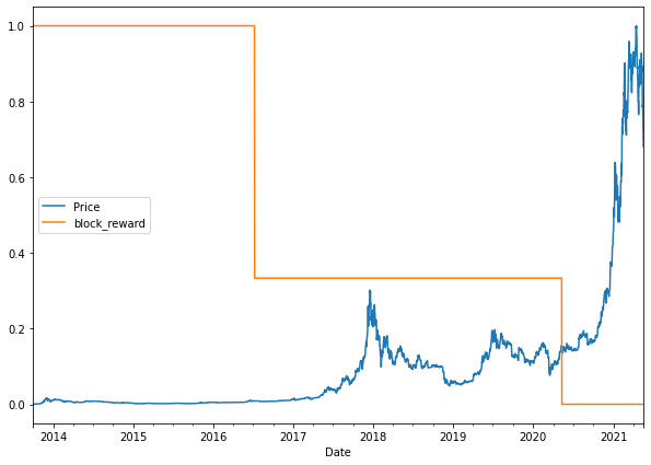
# Plot the block reward/price over time
# Note: Because of the different scales of our values we'll scale them to be between 0 and 1.
from sklearn.preprocessing import minmax_scale
scaled_price_block_df = pd.DataFrame(minmax_scale(bitcoin_prices_block[["Price", "block_reward"]]), # we need to scale the data first
                                     columns=bitcoin_prices_block.columns,
                                     index=bitcoin_prices_block.index)
scaled_price_block_df.plot(figsize=(10, 7));
Making a windowed dataset with pandas
Previously, we used some custom made functions to window our univariate time series.
However, since we’ve just added another variable to our dataset, these functions won’t work.
Not to worry though. Since our data is in a pandas DataFrame, we can leverage the pandas.DataFrame.shift() method to create a windowed multivariate time series.
The shift() method offsets an index by a specified number of periods.
# Setup dataset hyperparameters
HORIZON = 1
WINDOW_SIZE = 7
# Make a copy of the Bitcoin historical data with block reward feature
bitcoin_prices_windowed = bitcoin_prices_block.copy()

# Add windowed columns
for i in range(WINDOW_SIZE): # Shift values for each step in WINDOW_SIZE
  bitcoin_prices_windowed[f"Price+{i+1}"] = bitcoin_prices_windowed["Price"].shift(periods=i+1)
bitcoin_prices_windowed.head(10)
| Price | block_reward | Price+1 | Price+2 | Price+3 | Price+4 | Price+5 | Price+6 | Price+7 | |
|---|---|---|---|---|---|---|---|---|---|
| Date | |||||||||
| 2013-10-01 | 123.65499 | 25 | NaN | NaN | NaN | NaN | NaN | NaN | NaN |
| 2013-10-02 | 125.45500 | 25 | 123.65499 | NaN | NaN | NaN | NaN | NaN | NaN |
| 2013-10-03 | 108.58483 | 25 | 125.45500 | 123.65499 | NaN | NaN | NaN | NaN | NaN |
| 2013-10-04 | 118.67466 | 25 | 108.58483 | 125.45500 | 123.65499 | NaN | NaN | NaN | NaN |
| 2013-10-05 | 121.33866 | 25 | 118.67466 | 108.58483 | 125.45500 | 123.65499 | NaN | NaN | NaN |
| 2013-10-06 | 120.65533 | 25 | 121.33866 | 118.67466 | 108.58483 | 125.45500 | 123.65499 | NaN | NaN |
| 2013-10-07 | 121.79500 | 25 | 120.65533 | 121.33866 | 118.67466 | 108.58483 | 125.45500 | 123.65499 | NaN |
| 2013-10-08 | 123.03300 | 25 | 121.79500 | 120.65533 | 121.33866 | 118.67466 | 108.58483 | 125.45500 | 123.65499 |
| 2013-10-09 | 124.04900 | 25 | 123.03300 | 121.79500 | 120.65533 | 121.33866 | 118.67466 | 108.58483 | 125.45500 |
| 2013-10-10 | 125.96116 | 25 | 124.04900 | 123.03300 | 121.79500 | 120.65533 | 121.33866 | 118.67466 | 108.58483 |
# Let's create X & y, remove the NaN's and convert to float32 to prevent TensorFlow errors
X = bitcoin_prices_windowed.dropna().drop("Price", axis=1).astype(np.float32)
y = bitcoin_prices_windowed.dropna()["Price"].astype(np.float32)
X.head()
| block_reward | Price+1 | Price+2 | Price+3 | Price+4 | Price+5 | Price+6 | Price+7 | |
|---|---|---|---|---|---|---|---|---|
| Date | ||||||||
| 2013-10-08 | 25.0 | 121.794998 | 120.655327 | 121.338661 | 118.674660 | 108.584831 | 125.455002 | 123.654991 |
| 2013-10-09 | 25.0 | 123.032997 | 121.794998 | 120.655327 | 121.338661 | 118.674660 | 108.584831 | 125.455002 |
| 2013-10-10 | 25.0 | 124.049004 | 123.032997 | 121.794998 | 120.655327 | 121.338661 | 118.674660 | 108.584831 |
| 2013-10-11 | 25.0 | 125.961159 | 124.049004 | 123.032997 | 121.794998 | 120.655327 | 121.338661 | 118.674660 |
| 2013-10-12 | 25.0 | 125.279663 | 125.961159 | 124.049004 | 123.032997 | 121.794998 | 120.655327 | 121.338661 |
# View labels
y.head()
Date
2013-10-08    123.032997
2013-10-09    124.049004
2013-10-10    125.961159
2013-10-11    125.279663
2013-10-12    125.927498
Name: Price, dtype: float32
let’s split it into train and test sets using an 80/20 split just as we’ve done before.
# Make train and test sets
split_size = int(len(X) * 0.8)
X_train, y_train = X[:split_size], y[:split_size]
X_test, y_test = X[split_size:], y[split_size:]
len(X_train), len(y_train), len(X_test), len(y_test)
(2224, 2224, 556, 556)
Model 6: Dense (multivariate time series)
tf.random.set_seed(42)

# Make multivariate time series model
model_6 = tf.keras.Sequential([
  layers.Dense(128, activation="relu"),
  # layers.Dense(128, activation="relu"), # adding an extra layer here should lead to beating the naive model
  layers.Dense(HORIZON)
], name="model_6_dense_multivariate")

# Compile
model_6.compile(loss="mae",
                optimizer=tf.keras.optimizers.Adam())

# Fit
history_6 = model_6.fit(X_train, y_train,
                        epochs=100,
                        batch_size=128,
                        verbose=0, # only print 1 line per epoch
                        validation_data=(X_test, y_test),
                        callbacks=[create_model_checkpoint(model_name=model_6.name)])

plot_loss(history_6)
# Make sure best model is loaded and evaluate
model_6 = tf.keras.models.load_model("model_experiments/model_6_dense_multivariate")
model_6.evaluate(X_test, y_test)
18/18 [==============================] - 0s 2ms/step - loss: 568.0374


568.037353515625
# Make predictions on multivariate data
model_6_preds = tf.squeeze(model_6.predict(X_test))

# Evaluate preds
model_6_results = evaluate_preds(y_true=y_test,
                                 y_pred=model_6_preds)
MAE =  568.04
MSE =  1166217.2
RMSE =  1079.92
MAPE =  2.55
MASE =  1.0
model_1_results
{'mae': 585.9753,
 'mse': 1197801.1,
 'rmse': 1094.4409,
 'mape': 2.6149077,
 'mase': 1.0293963}
It looks like the adding in the block reward may have helped our model slightly.
Model 7: N-BEATS algorithm
So far we’ve tried a bunch of smaller models, models with only a couple of layers.
But one of the best ways to improve a model’s performance is to increase the number of layers in it.
That’s exactly what the N-BEATS (Neural Basis Expansion Analysis for Interpretable Time Series Forecasting) algorithm does.
The N-BEATS algorithm focuses on univariate time series problems and achieved state-of-the-art performance in the winner of the M4 competition (a forecasting competition).
For our next modelling experiment we’re going to be replicating the generic architecture of the N-BEATS algorithm (see section 3.3 of the N-BEATS paper).
We will focus on:
Replicating the model architecture in Figure 1 of the N-BEATS paper
Using the same hyperparameters as the paper which can be found in Appendix D of the N-BEATS paper
Doing this will give us an opportunity to practice:
- Creating a custom layer for the
NBeatsBlockby subclassingtf.keras.layers.Layer- Creating a custom layer is helpful for when TensorFlow doesn’t already have an existing implementation of a layer or if you’d like to make a layer configuration repeat a number of times (e.g. like a stack of N-BEATS blocks)
- Implementing a custom architecture using the Functional API
- Finding a paper related to our problem and seeing how it goes
# Create NBeatsBlock custom layer
class NBeatsBlock(tf.keras.layers.Layer):
  def __init__(self, # the constructor takes all the hyperparameters for the layer
               input_size: int,
               theta_size: int,
               horizon: int,
               n_neurons: int,
               n_layers: int,
               **kwargs): # the **kwargs argument takes care of all of the arguments for the parent class (input_shape, trainable, name)
    super().__init__(**kwargs)
    self.input_size = input_size
    self.theta_size = theta_size
    self.horizon = horizon
    self.n_neurons = n_neurons
    self.n_layers = n_layers

    # Block contains stack of 4 fully connected layers each has ReLU activation
    self.hidden = [tf.keras.layers.Dense(n_neurons, activation="relu") for _ in range(n_layers)]
    # Output of block is a theta layer with linear activation
    self.theta_layer = tf.keras.layers.Dense(theta_size, activation="linear", name="theta")

  def call(self, inputs): # the call method is what runs when the layer is called
    x = inputs
    for layer in self.hidden: # pass inputs through each hidden layer
      x = layer(x)
    theta = self.theta_layer(x)
    # Output the backcast and forecast from theta
    backcast, forecast = theta[:, :self.input_size], theta[:, -self.horizon:]
    return backcast, forecast
Setting up the NBeatsBlock custom layer we see:
- The class inherits from
tf.keras.layers.Layer(this gives it all of the methods assosciated withtf.keras.layers.Layer) - The constructor (
def __init__(...)) takes all of the layer hyperparameters as well as the**kwargsargument- The
**kwargsargument takes care of all of the hyperparameters which aren’t mentioned in the constructor such as,input_shape,trainableandname
- The
- In the constructor, the block architecture layers are created:
- The hidden layers are created as a stack of fully connected with
n_nueronshidden units layers with ReLU activation - The theta layer uses
theta_sizehidden units as well as linear activation
- The hidden layers are created as a stack of fully connected with
- The
call()method is what is run when the layer is called:- It first passes the inputs (the historical Bitcoin data) through each of the hidden layers (a stack of fully connected layers with ReLU activation)
- After the inputs have been through each of the fully connected layers, they get passed through the theta layer where the backcast (backwards predictions, shape:
input_size) and forecast (forward predictions, shape:horizon) are returned
Preparing data for the N-BEATS algorithm using tf.data
This time, because we are using a larger model architecture, to ensure our model training runs as fast as possible, we will setup our datasets using the tf.data API.
And because the N-BEATS algorithm is focused on univariate time series, we will start by making training and test windowed datasets of Bitcoin prices (just as we’ve done above).
HORIZON = 1 # how far to predict forward
WINDOW_SIZE = 7 # how far to lookback
# Create NBEATS data inputs (NBEATS works with univariate time series)
bitcoin_prices.head()
| Price | |
|---|---|
| Date | |
| 2013-10-01 | 123.65499 |
| 2013-10-02 | 125.45500 |
| 2013-10-03 | 108.58483 |
| 2013-10-04 | 118.67466 |
| 2013-10-05 | 121.33866 |
# Add windowed columns
bitcoin_prices_nbeats = bitcoin_prices.copy()
for i in range(WINDOW_SIZE):
  bitcoin_prices_nbeats[f"Price+{i+1}"] = bitcoin_prices_nbeats["Price"].shift(periods=i+1)
bitcoin_prices_nbeats.dropna().head()
| Price | Price+1 | Price+2 | Price+3 | Price+4 | Price+5 | Price+6 | Price+7 | |
|---|---|---|---|---|---|---|---|---|
| Date | ||||||||
| 2013-10-08 | 123.03300 | 121.79500 | 120.65533 | 121.33866 | 118.67466 | 108.58483 | 125.45500 | 123.65499 |
| 2013-10-09 | 124.04900 | 123.03300 | 121.79500 | 120.65533 | 121.33866 | 118.67466 | 108.58483 | 125.45500 |
| 2013-10-10 | 125.96116 | 124.04900 | 123.03300 | 121.79500 | 120.65533 | 121.33866 | 118.67466 | 108.58483 |
| 2013-10-11 | 125.27966 | 125.96116 | 124.04900 | 123.03300 | 121.79500 | 120.65533 | 121.33866 | 118.67466 |
| 2013-10-12 | 125.92750 | 125.27966 | 125.96116 | 124.04900 | 123.03300 | 121.79500 | 120.65533 | 121.33866 |
# Make features and labels
X = bitcoin_prices_nbeats.dropna().drop("Price", axis=1)
y = bitcoin_prices_nbeats.dropna()["Price"]

# Make train and test sets
split_size = int(len(X) * 0.8)
X_train, y_train = X[:split_size], y[:split_size]
X_test, y_test = X[split_size:], y[split_size:]
len(X_train), len(y_train), len(X_test), len(y_test)
(2224, 2224, 556, 556)
- Turning the arrays in tensor Datasets using
tf.data.Dataset.from_tensor_slices()
- Note:
from_tensor_slices()works best when your data fits in memory, for extremely large datasets, you’ll want to look into using theTFRecordformat
- Combine the labels and features tensors into a Dataset using
tf.data.Dataset.zip() - Batch and prefetch the Datasets using
batch()andprefetch()
- Batching and prefetching ensures the loading time from CPU (preparing data) to GPU (computing on data) is as small as possible
# 1. Turn train and test arrays into tensor Datasets
train_features_dataset = tf.data.Dataset.from_tensor_slices(X_train)
train_labels_dataset = tf.data.Dataset.from_tensor_slices(y_train)

test_features_dataset = tf.data.Dataset.from_tensor_slices(X_test)
test_labels_dataset = tf.data.Dataset.from_tensor_slices(y_test)

# 2. Combine features & labels
train_dataset = tf.data.Dataset.zip((train_features_dataset, train_labels_dataset))
test_dataset = tf.data.Dataset.zip((test_features_dataset, test_labels_dataset))

# 3. Batch and prefetch for optimal performance
BATCH_SIZE = 1024 # taken from Appendix D in N-BEATS paper
train_dataset = train_dataset.batch(BATCH_SIZE).prefetch(tf.data.AUTOTUNE)
test_dataset = test_dataset.batch(BATCH_SIZE).prefetch(tf.data.AUTOTUNE)

train_dataset, test_dataset
(<PrefetchDataset element_spec=(TensorSpec(shape=(None, 7), dtype=tf.float64, name=None), TensorSpec(shape=(None,), dtype=tf.float64, name=None))>,
 <PrefetchDataset element_spec=(TensorSpec(shape=(None, 7), dtype=tf.float64, name=None), TensorSpec(shape=(None,), dtype=tf.float64, name=None))>)
Data prepared! Notice the input shape for the features (None, 7), the None leaves space for the batch size where as the 7 represents the WINDOW_SIZE.
Time to get create the N-BEATS architecture.
# Model hyper parameters
# Values from N-BEATS paper Figure 1 and Table 18/Appendix D
N_EPOCHS = 5000 # called "Iterations" in Table 18
N_NEURONS = 512 # called "Width" in Table 18
N_LAYERS = 4
N_STACKS = 30

INPUT_SIZE = WINDOW_SIZE * HORIZON # called "Lookback" in Table 18
THETA_SIZE = INPUT_SIZE + HORIZON

INPUT_SIZE, THETA_SIZE
(7, 8)
Residual connections
double residual stacking (section 3.2 of the N-BEATS paper):
tf.keras.layers.subtract(inputs)- subtracts list of input tensors from each othertf.keras.layers.add(inputs)- adds list of input tensors to each other
# Make tensors
tensor_1 = tf.range(10) + 10
tensor_2 = tf.range(10)

# Subtract
subtracted = layers.subtract([tensor_1, tensor_2])

# Add
added = layers.add([tensor_1, tensor_2])

print(f"Input tensors: {tensor_1.numpy()} & {tensor_2.numpy()}")
print(f"Subtracted: {subtracted.numpy()}")
print(f"Added: {added.numpy()}")
Input tensors: [10 11 12 13 14 15 16 17 18 19] & [0 1 2 3 4 5 6 7 8 9]
Subtracted: [10 10 10 10 10 10 10 10 10 10]
Added: [10 12 14 16 18 20 22 24 26 28]
The power of residual stacking or residual connections was revealed in Deep Residual Learning for Image Recognition where the authors were able to build a deeper but less complex neural network (this is what introduced the popular ResNet architecture) than previous attempts.
This deeper neural network led to state of the art results on the ImageNet challenge in 2015 and different versions of residual connections have been present in deep learning ever since.
A residual connection (also called skip connections) involves a deeper neural network layer receiving the outputs as well as the inputs of a shallower neural network layer.
In the case of N-BEATS, the architecture uses residual connections which:
- Subtract the backcast outputs from a previous block from the backcast inputs to the current block
- Add the forecast outputs from all blocks together in a stack
In practice, residual connections have been beneficial for training deeper models (N-BEATS reaches ~150 layers, also see “These approaches provide clear advantages in improving the trainability of deep architectures” in section 3.2 of the N-BEATS paper).
It’s thought that they help avoid the problem of vanishing gradients (patterns learned by a neural network not being passed through to deeper layers).
 %%time

tf.random.set_seed(42)

# 1. Setup N-BEATS Block layer
nbeats_block_layer = NBeatsBlock(input_size=INPUT_SIZE,
                                 theta_size=THETA_SIZE,
                                 horizon=HORIZON,
                                 n_neurons=N_NEURONS,
                                 n_layers=N_LAYERS,
                                 name="InitialBlock")

# 2. Create input to stacks
stack_input = layers.Input(shape=(INPUT_SIZE), name="stack_input")

# 3. Create initial backcast and forecast input (backwards predictions are referred to as residuals in the paper)
backcast, forecast = nbeats_block_layer(stack_input)
# Add in subtraction residual link, thank you to: https://github.com/mrdbourke/tensorflow-deep-learning/discussions/174
residuals = layers.subtract([stack_input, backcast], name=f"subtract_00")

# 4. Create stacks of blocks
for i, _ in enumerate(range(N_STACKS-1)): # first stack is already creted in (3)

  # 5. Use the NBeatsBlock to calculate the backcast as well as block forecast
  backcast, block_forecast = NBeatsBlock(
      input_size=INPUT_SIZE,
      theta_size=THETA_SIZE,
      horizon=HORIZON,
      n_neurons=N_NEURONS,
      n_layers=N_LAYERS,
      name=f"NBeatsBlock_{i}"
  )(residuals) # pass it in residuals (the backcast)

  # 6. Create the double residual stacking
  residuals = layers.subtract([residuals, backcast], name=f"subtract_{i}")
  forecast = layers.add([forecast, block_forecast], name=f"add_{i}")

# 7. Put the stack model together
model_7 = tf.keras.Model(inputs=stack_input,
                         outputs=forecast,
                         name="model_7_N-BEATS")

# 8. Compile with MAE loss and Adam optimizer
model_7.compile(loss="mae",
                optimizer=tf.keras.optimizers.Adam(0.001),
                metrics=["mae", "mse"])

# 9. Fit the model with EarlyStopping and ReduceLROnPlateau callbacks
history_7 = model_7.fit(train_dataset,
                        epochs=N_EPOCHS,
                        validation_data=test_dataset,
                        verbose=0, # prevent large amounts of training outputs
                        # callbacks=[create_model_checkpoint(model_name=stack_model.name)] # saving model every epoch consumes far too much time
                        callbacks=[tf.keras.callbacks.EarlyStopping(monitor="val_loss", patience=200, restore_best_weights=True),
                                  tf.keras.callbacks.ReduceLROnPlateau(monitor="val_loss", patience=100, verbose=1)])
Epoch 191: ReduceLROnPlateau reducing learning rate to 0.00010000000474974513.

Epoch 300: ReduceLROnPlateau reducing learning rate to 1.0000000474974514e-05.

Epoch 400: ReduceLROnPlateau reducing learning rate to 1.0000000656873453e-06.
CPU times: user 1min 4s, sys: 1.7 s, total: 1min 6s
Wall time: 1min 10s
plot_loss(history_6)

# Make predictions with N-BEATS model
model_7_preds = make_preds(model_7, test_dataset)

# Evaluate N-BEATS model predictions
model_7_results = evaluate_preds(y_true=y_test,
                                 y_pred=model_7_preds)
MAE =  574.98
MSE =  1191869.9
RMSE =  1091.73
MAPE =  2.66
MASE =  1.01
# Plot the N-BEATS model and inspect the architecture
from tensorflow.keras.utils import plot_model
plot_model(model_7)
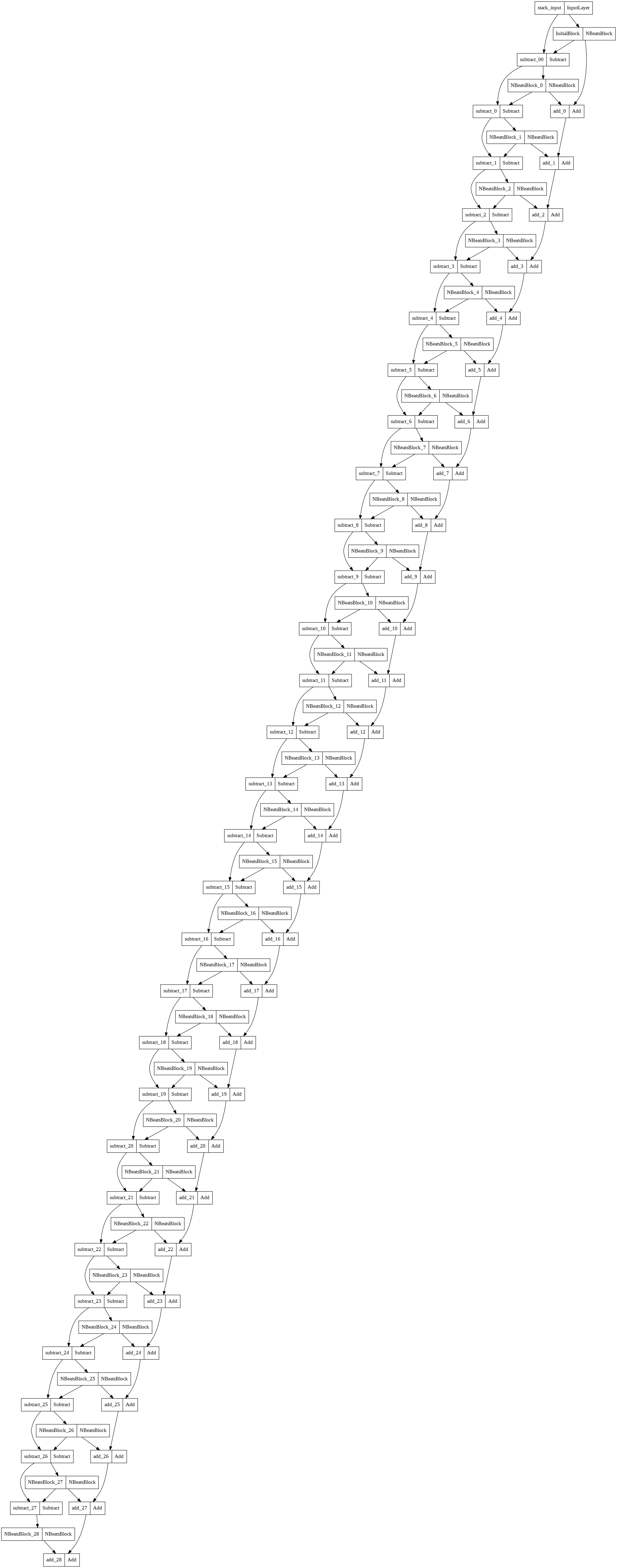
Model 8: Train a model on the full historical data to make predictions into future
bitcoin_prices_windowed.head()
| Price | block_reward | Price+1 | Price+2 | Price+3 | Price+4 | Price+5 | Price+6 | Price+7 | |
|---|---|---|---|---|---|---|---|---|---|
| Date | |||||||||
| 2013-10-01 | 123.65499 | 25 | NaN | NaN | NaN | NaN | NaN | NaN | NaN |
| 2013-10-02 | 125.45500 | 25 | 123.65499 | NaN | NaN | NaN | NaN | NaN | NaN |
| 2013-10-03 | 108.58483 | 25 | 125.45500 | 123.65499 | NaN | NaN | NaN | NaN | NaN |
| 2013-10-04 | 118.67466 | 25 | 108.58483 | 125.45500 | 123.65499 | NaN | NaN | NaN | NaN |
| 2013-10-05 | 121.33866 | 25 | 118.67466 | 108.58483 | 125.45500 | 123.65499 | NaN | NaN | NaN |
# Train model on entire data to make prediction for the next day
X_all = bitcoin_prices_windowed.drop(["Price", "block_reward"], axis=1).dropna().to_numpy() # only want prices, our future model can be a univariate model
y_all = bitcoin_prices_windowed.dropna()["Price"].to_numpy()
# 1. Turn X and y into tensor Datasets
features_dataset_all = tf.data.Dataset.from_tensor_slices(X_all)
labels_dataset_all = tf.data.Dataset.from_tensor_slices(y_all)

# 2. Combine features & labels
dataset_all = tf.data.Dataset.zip((features_dataset_all, labels_dataset_all))

# 3. Batch and prefetch for optimal performance
BATCH_SIZE = 1024 # taken from Appendix D in N-BEATS paper
dataset_all = dataset_all.batch(BATCH_SIZE).prefetch(tf.data.AUTOTUNE)

dataset_all
<PrefetchDataset element_spec=(TensorSpec(shape=(None, 7), dtype=tf.float64, name=None), TensorSpec(shape=(None,), dtype=tf.float64, name=None))>
tf.random.set_seed(42)

# Create model (nice and simple, just to test)
model_8 = tf.keras.Sequential([
  layers.Dense(128, activation="relu"),
  layers.Dense(128, activation="relu"),
  layers.Dense(HORIZON)
])

# Compile
model_8.compile(loss=tf.keras.losses.mae,
                optimizer=tf.keras.optimizers.Adam())

# Fit model on all of the data to make future forecasts
history_8 = model_8.fit(dataset_all,
                        epochs=100,
                        verbose=0) # don't print out anything, we've seen this all before
  plt.figure(figsize=(10, 7))
  plt.plot(history_8.history['loss'], label = "loss")
  plt.xlabel("Epochs")
  plt.ylabel("loss")
  plt.legend()
  plt.show()
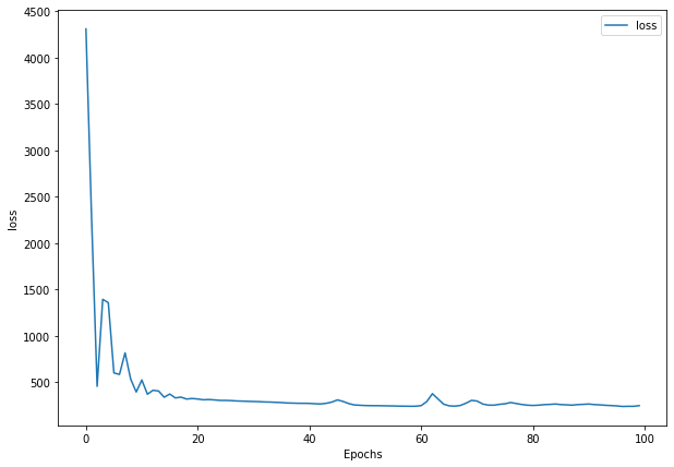
# How many timesteps to predict into the future?
INTO_FUTURE = 12*7 # since our Bitcoin data is daily, this is for three month
We will build the following steps:
- Function which takes as input:
- a list of values (the Bitcoin historical data)
- a trained model (such as
model_9) - a window into the future to predict (our
INTO_FUTUREvariable) - the window size a model was trained on (
WINDOW_SIZE) - the model can only predict on the same kind of data it was trained on
- Creates an empty list for future forecasts (this will be returned at the end of the function) and extracts the last
WINDOW_SIZEvalues from the input values (predictions will start from the lastWINDOW_SIZEvalues of the training data) - Loop
INTO_FUTUREtimes making a prediction onWINDOW_SIZEdatasets which update to remove the first the value and append the latest prediction
- Eventually future predictions will be made using the model’s own previous predictions as input
# 1. Create function to make predictions into the future
def make_future_forecast(values, model, into_future, window_size=WINDOW_SIZE) -> list:
  """
  Makes future forecasts into_future steps after values ends.

  Returns future forecasts as list of floats.
  """
  # 2. Make an empty list for future forecasts/prepare data to forecast on
  future_forecast = []
  last_window = values[-WINDOW_SIZE:] # only want preds from the last window (this will get updated)

  # 3. Make INTO_FUTURE number of predictions, altering the data which gets predicted on each time
  for _ in range(into_future):

    # Predict on last window then append it again, again, again (model starts to make forecasts on its own forecasts)
    future_pred = model.predict(tf.expand_dims(last_window, axis=0))
    # print(f"Predicting on: \n {last_window} -> Prediction: {tf.squeeze(future_pred).numpy()}\n")

    # Append predictions to future_forecast
    future_forecast.append(tf.squeeze(future_pred).numpy())
    # print(future_forecast)

    # Update last window with new pred and get WINDOW_SIZE most recent preds (model was trained on WINDOW_SIZE windows)
    last_window = np.append(last_window, future_pred)[-WINDOW_SIZE:]

  return future_forecast
# Make forecasts into future of the price of Bitcoin
# Note: if you're reading this at a later date, you may already be in the future, so the forecasts
# we're making may not actually be forecasts, if that's the case, readjust the training data.
future_forecast = make_future_forecast(values=y_all,
                                       model=model_8,
                                       into_future=INTO_FUTURE,
                                       window_size=WINDOW_SIZE)
def get_future_dates(start_date, into_future, offset=1):
  """
  Returns array of datetime values from ranging from start_date to start_date+horizon.

  start_date: date to start range (np.datetime64)
  into_future: number of days to add onto start date for range (int)
  offset: number of days to offset start_date by (default 1)
  """
  start_date = start_date + np.timedelta64(offset, "D") # specify start date, "D" stands for day
  end_date = start_date + np.timedelta64(into_future, "D") # specify end date
  return np.arange(start_date, end_date, dtype="datetime64[D]") # return a date range between start date and end date
# Last timestep of timesteps (currently in np.datetime64 format)
last_timestep = bitcoin_prices.index[-1]
last_timestep
Timestamp('2021-05-18 00:00:00')
# Get next two weeks of timesteps
next_time_steps = get_future_dates(start_date=last_timestep,
                                   into_future=INTO_FUTURE)
But to make sure the lines of the plot connect (try not running the cell below and then plotting the data to see what I mean), let’s insert the last timestep and Bitcoin price of our training data to the next_time_steps and future_forecast arrays.
# Insert last timestep/final price so the graph doesn't look messed
next_time_steps = np.insert(next_time_steps, 0, last_timestep)
future_forecast = np.insert(future_forecast, 0, prices[-1])
# Plot future price predictions of Bitcoin
plt.figure(figsize=(10, 7))
plot_time_series(bitcoin_prices.index, prices, start=2500, format="-", label="Actual BTC Price")
plot_time_series(next_time_steps, future_forecast, format="-", label="Predicted BTC Price")
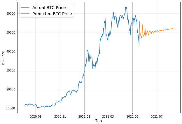
Compare Models
# Compare different model results (w = window, h = horizon, e.g. w=7 means a window size of 7)
model_results = pd.DataFrame({"naive_model": naive_results,
                              "model_1_dense_w7_h1": model_1_results,
                              "model_2_dense_w30_h1": model_2_results,
                              "model_3_dense_w30_h7": model_3_results,
                              "model_4_CONV1D": model_4_results,
                              "model_5_LSTM": model_5_results,
                              "model_6_multivariate": model_6_results,
                              "model_8_NBEATs": model_7_results}).T
model_results.head(10)
| mae | mse | rmse | mape | mase | |
|---|---|---|---|---|---|
| naive_model | 567.980225 | 1147547.000 | 1071.236206 | 2.516525 | 0.999570 |
| model_1_dense_w7_h1 | 585.975281 | 1197801.125 | 1094.440918 | 2.614908 | 1.029396 |
| model_2_dense_w30_h1 | 608.961975 | 1281440.625 | 1132.007324 | 2.769341 | 1.064471 |
| model_3_dense_w30_h7 | 748.776917 | 1690645.625 | 812.749695 | 3.539839 | 1.308869 |
| model_4_CONV1D | 610.154236 | 1242911.125 | 1114.859253 | 2.756886 | 1.071872 |
| model_5_LSTM | 597.462341 | 1275416.000 | 1129.343140 | 2.691097 | 1.049576 |
| model_6_multivariate | 568.037292 | 1166217.250 | 1079.915405 | 2.546613 | 0.997884 |
| model_8_NBEATs | 574.983643 | 1191869.875 | 1091.727905 | 2.663940 | 1.010087 |
# Sort model results by MAE and plot them
model_results[["mae"]].sort_values(by="mae").plot(figsize=(10, 7), kind="bar");